当需要大量通过程序计算,还要绘制图像才可以查看计算结果的时候, 利用Origin绘图显得非常耗时, 所以这里就想把自己通常用到的数据格式, 通过gnuplot来绘制结果, 这样可以在之后的计算研究过程中, 直接通过代码作图, 从而节省时间, 毕竟时间是最重要的东西.
2D密度图
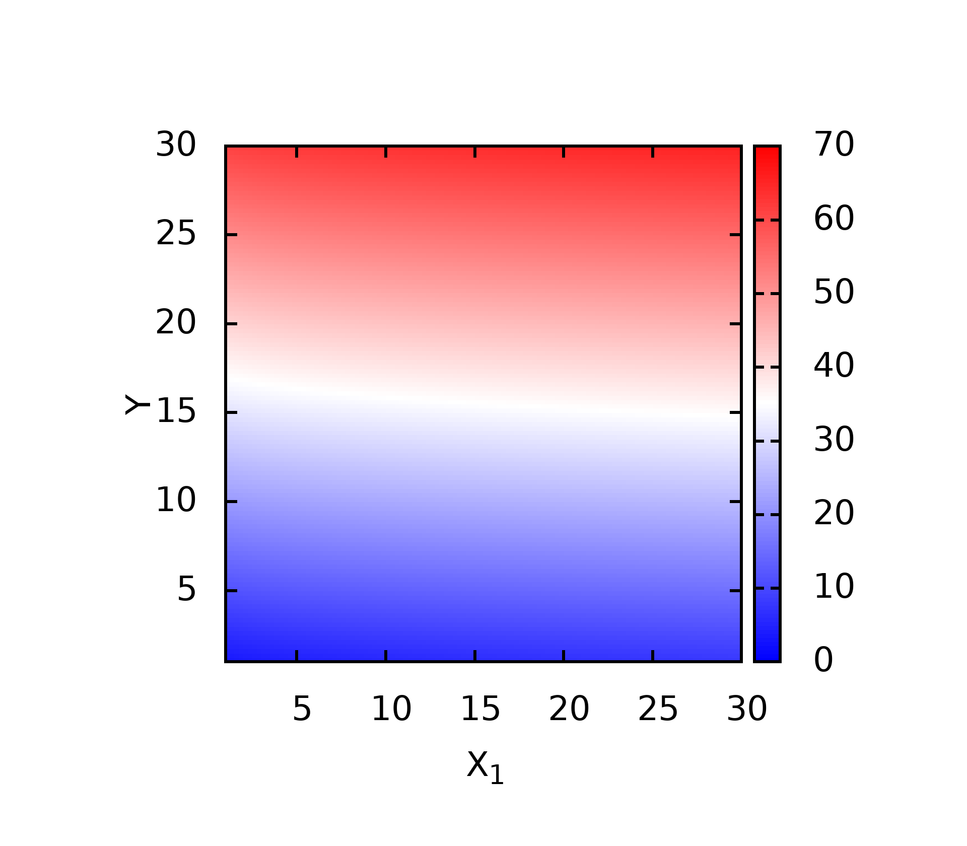
首先通过下面的fortran代码来展示出通过gnuplot来画密度图, 所欲要的数据格式是什么样的, 然后再利用gnuplot来绘图
program main
implicit none
integer ne
ne = 100
call main1(ne)
stop
end
!=================================
subroutine main1(ne)
implicit none
integer i,j,k,ne
real r1,r2
open(10,file="test.dat")
do i = 1,ne
    do j = 1,ne
       write(10,*)i,j,sqrt(1.0*i) + 2.0*j
    end do
    write(10,*)
end do
close(10)
end subroutine
这里在绘图的时候, 需要在每隔一定的数据间隔后加一个空行, 才可以实现.

在程序计算的时候, 将数据保存成上面需要的形式之后, 就可以利用gnuplot来进行绘图
set encoding iso_8859_1
#set terminal  postscript enhanced color
#set output 'arc_r.eps'
#set terminal pngcairo truecolor enhanced  font ",50" size 1920, 1680
set terminal png truecolor enhanced font ",50" size 1920, 1680
set output 'density.png'
#set palette defined ( -10 "#194eff", 0 "white", 10 "red" )  # 密度图颜色设置
set palette defined ( -10 "blue", 0 "white", 10 "red" )
#set palette rgbformulae 33,13,10
unset ztics
unset key
set pm3d
set border lw 6
set size ratio -1
set view map
set xtics
set ytics
#set xlabel "K_1 (1/{\305})"  # 坐标轴标签设置
set xlabel "X_1"
#set ylabel "K_2 (1/{\305})"
set ylabel "Y"
set ylabel offset 1, 0
set colorbox
set xrange [1: 30]
set yrange [1: 30]
set pm3d interpolate 4,4   # 设置插值,让图像变得更加平滑
splot 't3.dat' u 1:2:3 w pm3d
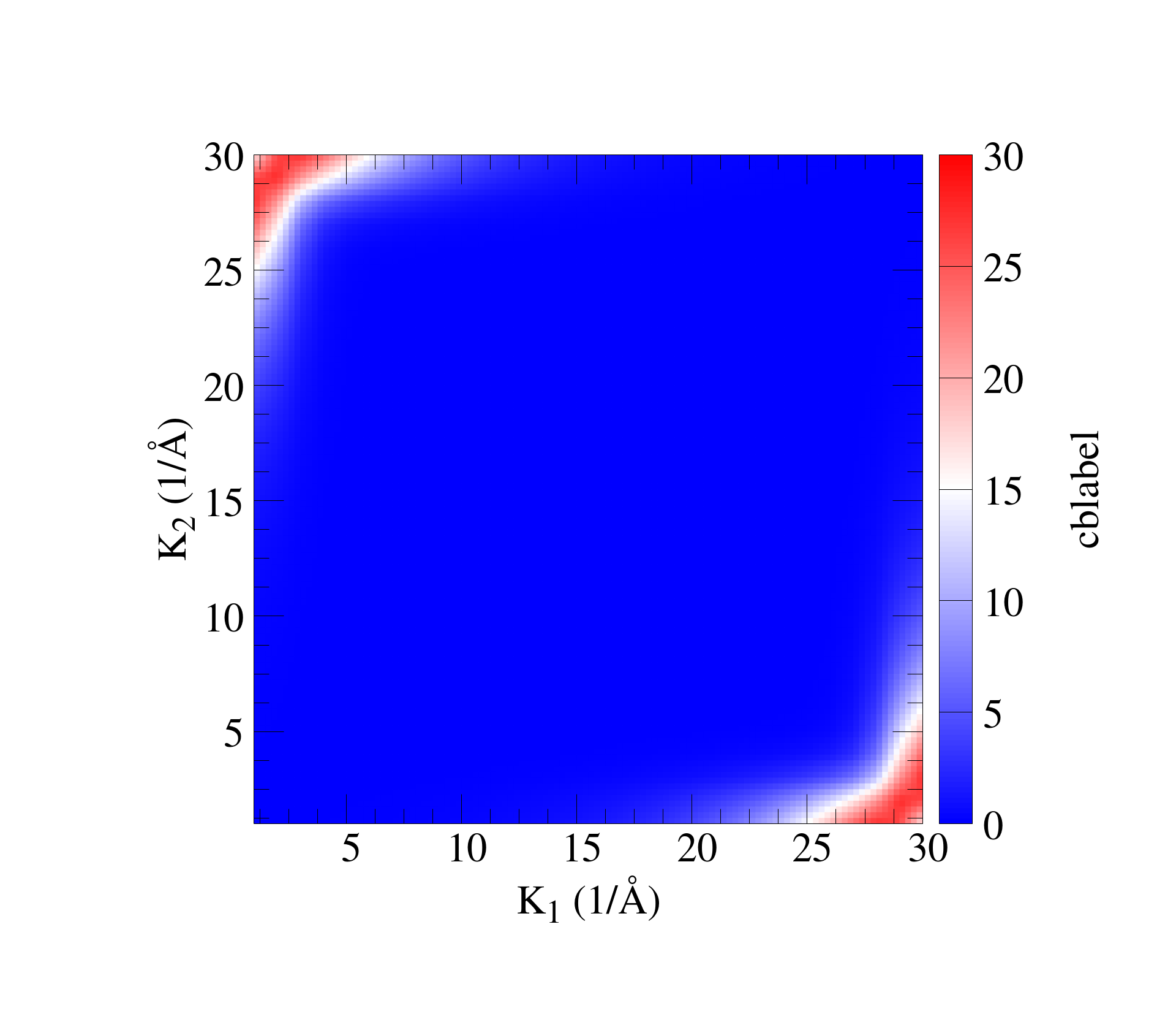
- 升级版
 set encoding iso_8859_1
 #set terminal  postscript enhanced color
 #set output 'arc_r.eps'
 #set terminal pngcairo truecolor enhanced  font ",50" size 1920, 1680
 set terminal png truecolor enhanced font ",50" size 1920, 1680
 set output 'm01_oxy.png'
 #set palette defined ( -10 "#194eff", 0 "white", 10 "red" )
 set palette defined ( -10 "blue", 0 "white", 10 "red" )
 #set palette rgbformulae 33,13,10
 unset ztics
 unset key
 set pm3d
 #set border lw 6
 set size ratio -1
 set view map
 set xtics
 set ytics
 set xlabel "K_1 (1/{\305})" font 'Times,Bold' offset 0,1.5
 #set xlabel "X"
 set ylabel "K_2 (1/{\305})" font 'Times,Bold' offset 1.5,0
 #set xlabel "X"
 #set ylabel "Y"
 #set ylabel offset 1, 0
 #set xlabel offset 0, 1
 set ytics offset 1,0 font 'Times,Bold'
 set xtics offset 0,1 font 'Times,Bold'
 set mxtics 4
 set mytics 4
 set colorbox
 set cblabel 'cblabel' font 'Times,Bold'
 set cbtics offset -1,0  font 'Times,Bold'
 set xrange [1: 30]
 set yrange [1: 30]
 set pm3d interpolate 4,4
 splot 'ldos-diag01.dat' u 1:2:3 w pm3d
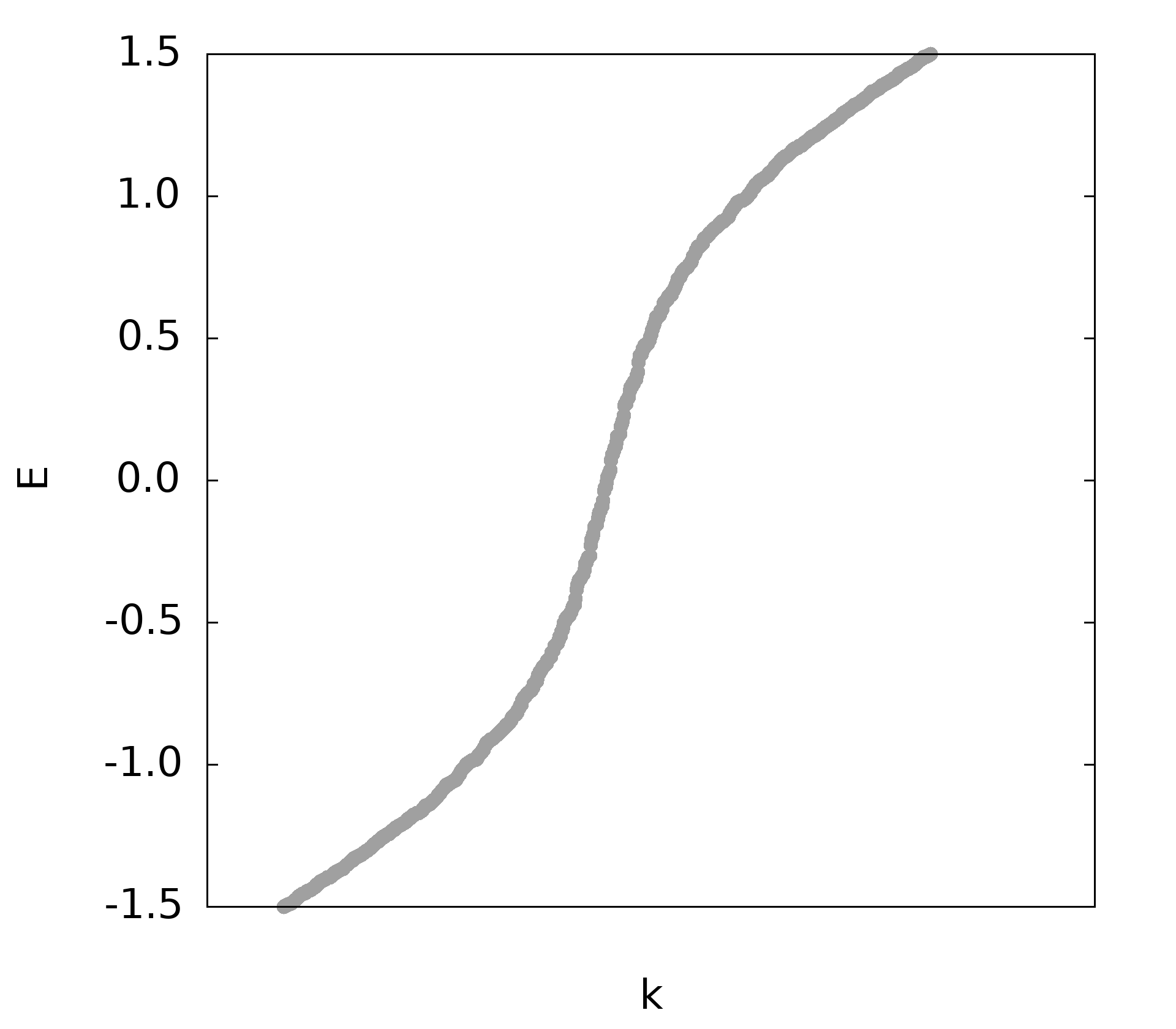
1d散点图
三点图没太多需要说明的, 就是最简单的一维数据点绘图
set encoding iso_8859_1
#set terminal  postscript enhanced color font ",30"  # Set for eps formation
#set output 'wcc.eps'
set terminal png truecolor enhanced font ",50" size 1920, 1680 # Set for png formation
set output 'eigval.png'
unset key
set border lw 3
set xtics offset 0, 0.0
set xtics format "%4.1f" nomirror out
#set xlabel '{/symbol eta}'
set xlabel 'k'
set xlabel offset 0, -1.0
set ytics 0.5
unset xtics
#set ytics format "%4.1f" nomirror out
set ytics format "%4.1f"
set ylabel "E"
set ylabel offset 0.5, 0.0
set xrange [3550: 3650]
set yrange [-1.5:1.5]
#plot for [i=4:     4] 'wcc.dat' u 1:i w p  pt 7  ps 1.1 lc 'red'
plot 'eigval.dat' u 1:2 w p pt 7 ps 4 lc 'red'
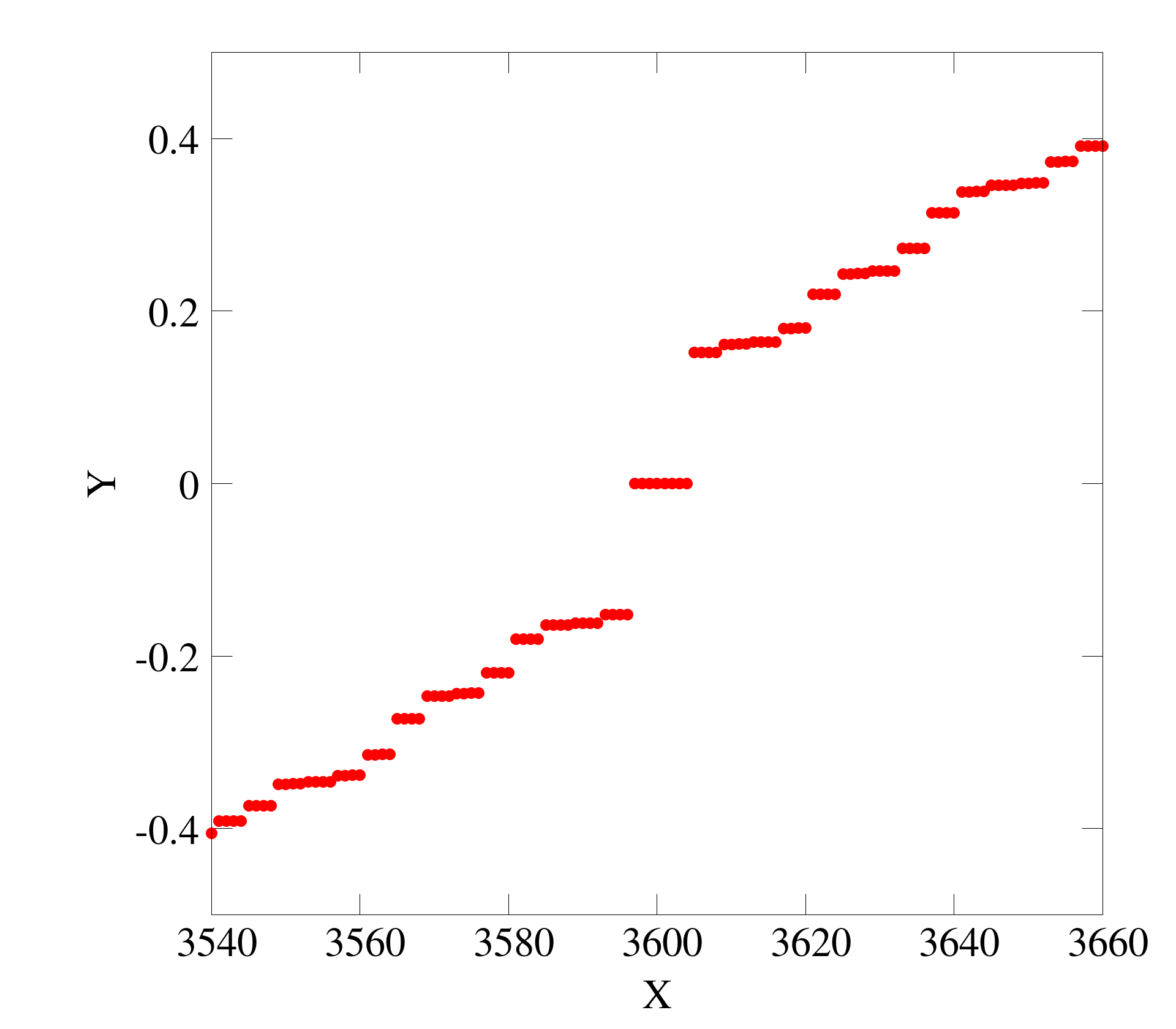
- 升级版
 set encoding iso_8859_1
 #set terminal  postscript enhanced color
 #set output 'arc_r.eps'
 #set terminal pngcairo truecolor enhanced  font ",50" size 1920, 1680
 set terminal png truecolor enhanced font ",50" size 1920, 1680
 set output 'm01_val.png'
 unset key
 set xlabel "X" font "Times,Bold" offset 0,1.0
 set ylabel "Y" font "Times,Bold" offset 1.5,0
 set ytics offset 0.5,0 font "Times,Bold"
 set xtics offset 0,0.5 font "Times,Bold"
 set xrange [3540:3660]
 set yrange [-0.5:0.5]
 plot 'eigval-diag01.dat' u 1:2 ps 3.0 pt 7
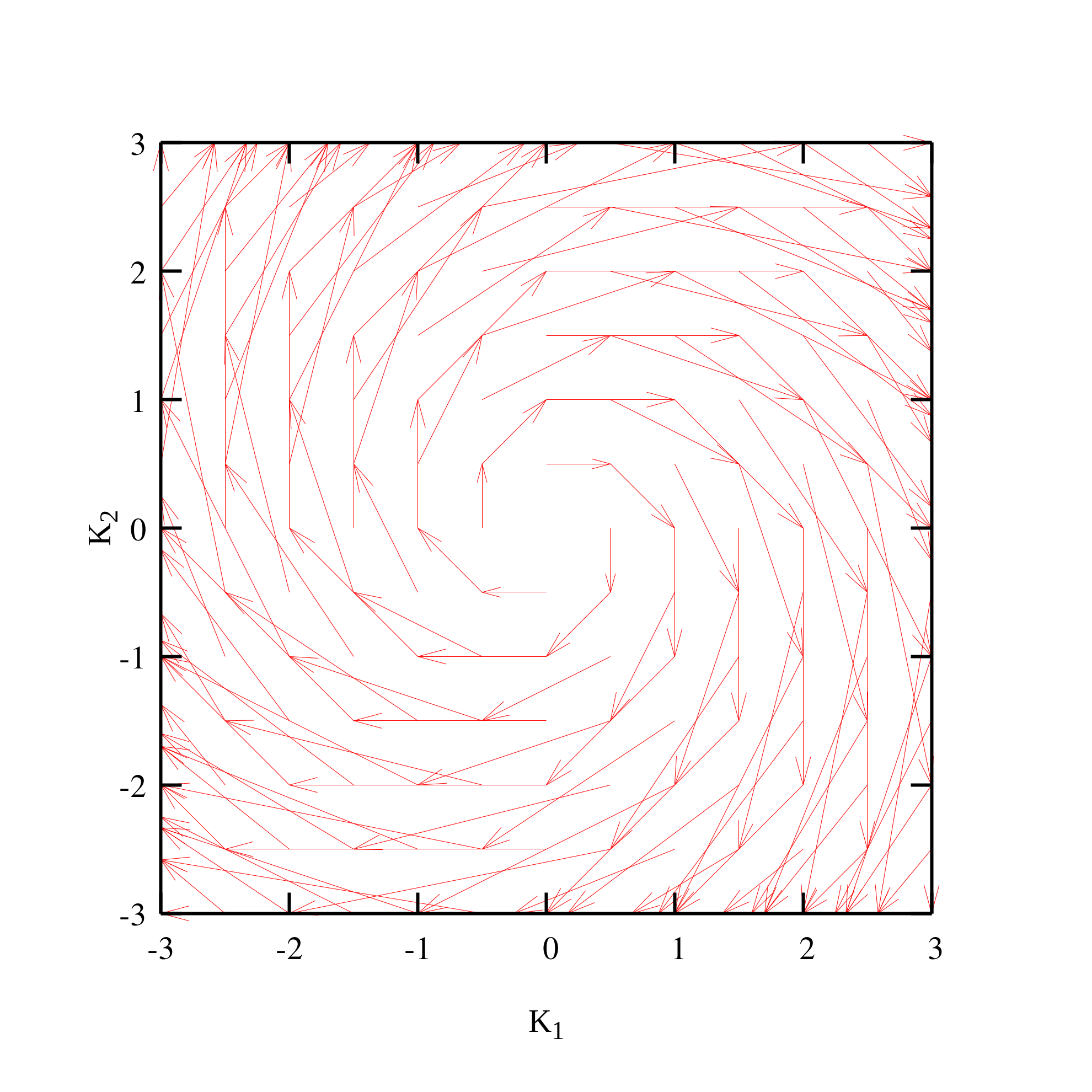
矢量场图
先利用Fortran产生数据
   program main
   implicit none
   integer i1,i2,i3,num
   real r1,r2,r3
   open(10,file="vec.dat")
   do r1 = -3,3,0.5
      do r2 = -3,3,0.5
         write(10,999)r1,r2,r2,-r1
      end do
   end do
   close(10)
999format(8f11.5)
   stop
   end program main
再利用gnuplot进行绘图
set encoding iso_8859_1
set terminal  pngcairo truecolor enhanced lw 1.0 font "TimesNewRoman, 44" size 1980,1980
set output 'testure.png'
set xlabel 'K_1'
set ylabel 'K_2'
unset key
set pm3d
set border lw 6
set ytics offset 0.5,0 font "Times,Bold"
set xtics offset 0,0.5 font "Times,Bold"
set size ratio 1
set view map
unset colorbox
set xrange [-3:3]
set yrange [-3:3]
splot 'vec.dat' u 1:2:(0):3:4:(0)  w vec  head lw 1
绘图设置
set term pdfcairo lw 2 font "Times New Roman,8" # 设置输出pdf格式,使用字体为Times New Roman, 字体大小为8
set terminal postscript eps color solid linewidth 2 # 设置输出eps图片, color为彩图输出
set term pngcairo lw 2 font "AR PL UKai CN,14"  # 设置输出png图片
set output 'test.pdf' # 设置输出文件名
plot 'test.dat' u 1:4 w lp pt 5,'test.dat' u 1:3 w lp pt 7  # 绘图
set output # 输出
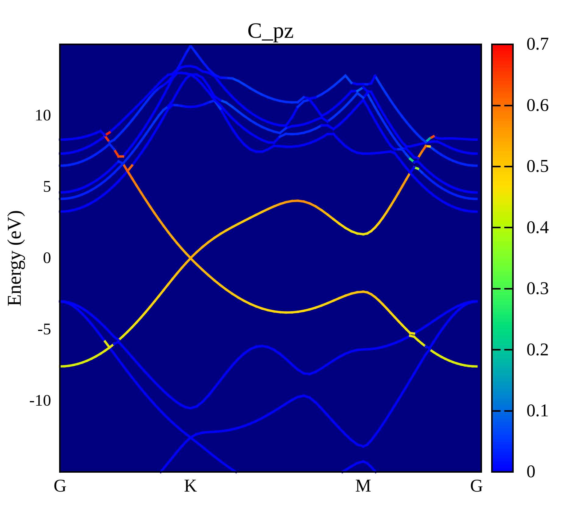
投影能带图
set encoding iso_8859_1
#set terminal  postscript enhanced color font "TimesNewRoman, 11" size 5, 4
set terminal  pngcairo truecolor enhanced lw 5.0 font "TimesNewRoman, 44" size 1920, 1680
set palette rgbformulae 22, 13, -31
# # set palette rgbformulae 7,5,15
set output 'C_pz.png'
set border
# unset colorbox
set title "C\\_pz" offset 0, -0.8 font "TimesNewRoman, 54"
set style data linespoints
unset ztics
unset key
# # set key outside top vertical center
# # set pointsize 0.3
set view 0,0
set xtics font "TimesNewRoman, 44"
set xtics offset 0, 0.3
set ytics font "TimesNewRoman, 40"
set ytics -10, 5, 10
set ylabel font "TimesNewRoman, 48"
set ylabel offset 1.0, 0
set xrange [0:5.4704]
set ylabel "Energy (eV)"
set yrange [-15:15]
set xtics ("G" 0.00000, "K" 1.695, "M" 3.938, "G" 5.407)
plot -10 with filledcurves y1=10 lc rgb "navy", \
'PBAND_C.dat' u ($1):($2):($5) w lines lw 1.5 lc palette
这个程序是我从使用gnuplot画投影能带图这篇博客中找到的,利用这个模板绘制了Graphene的能带
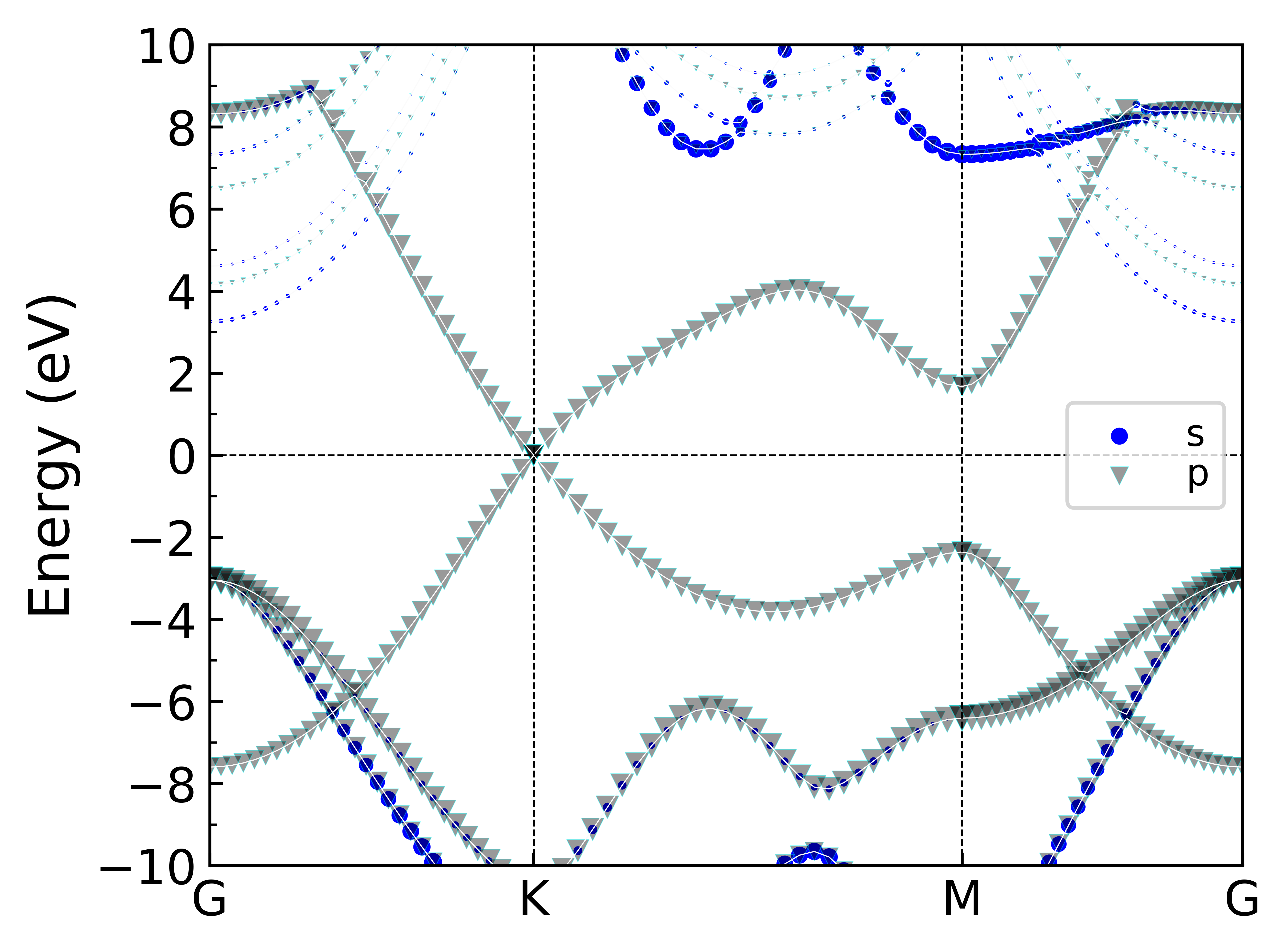
python同样也可以绘制相同的图片,不过相比较而言,找到的Python这个绘图模板可以同时对多个原子的投影轨道进行绘制
#!/usr/bin/python
# -*- coding:utf-8 -*-

"""
@author: V. Wang, Jin-Cheng Liu, Nxu
@file: pband_plot.py
@time: 2018/12/18 20:57
A script to plot PBAND
modified some details by He Yong
"""

import numpy as np
import matplotlib as mpl
import os
mpl.use('Agg')  # silent mode
from matplotlib import pyplot as plt
import matplotlib.ticker as ticker
import sys

#------------------- rc.Params 1----------------------
plt.rcParams['xtick.direction'] = 'in'
plt.rcParams['ytick.direction'] = 'in'

#------------------- Data Read ----------------------

def getelementinfo():
    try:
        with open("POSCAR",'r') as reader:
            line_s=reader.readlines()
    except:
        print("No POSCAR found!")
    try:
        element_s=line_s[5].rstrip('\r\n').rstrip('\n')
        elements=element_s.split()
    except:
        print("POSCAR element line is wrong!")

    data = {}
    for i in range(len(elements)):
        data[elements[i]]=np.loadtxt("PBAND_" + elements[i] + ".dat")
    return data,elements

def getHighSymmetryPoints():
    hsp = np.loadtxt("KLABELS", dtype=np.string_, skiprows=1, usecols=(0, 1))
    group_labels = hsp[:-1, 0].tolist()
    group_labels = [i.decode('utf-8', 'ignore') for i in group_labels]
    for index in range(len(group_labels)):
        if group_labels[index] == "GAMMA":
            group_labels[index] = u"Γ"
    return group_labels, hsp


def maxminnorm(a):
    amin, amax = a.min(), a.max()  # fin maximum minimum
    if amax == 0:
        return a
    else:
        a = (a - amin) / (amax - amin)  # (value-minimum)/(maximum-minimum)
        return a


def getPbandData(data, scaler):
    kpt = data[:, 0]  # kpath
    eng = data[:, 1]  # energy level
    wgt_s = data[:, 2] * scaler  # weight, 20 is enlargement factor
    #wgt_s = maxminnorm(wgt_s) * scaler  # Normlized

    wgt_py = data[:, 3] * scaler  # weight, 20 is enlargement factor
    #wgt_py = maxminnorm(wgt_py)*scaler
    wgt_pz = data[:, 4] * scaler  # weight, 20 is enlargement factor
    #wgt_pz = maxminnorm(wgt_pz)*scaler

    wgt_px = data[:, 5] * scaler  # weight, 20 is enlargement factor
    #wgt_px = maxminnorm(wgt_px)*scaler

    wgt_p = np.array(wgt_py) + np.array(wgt_px) + np.array(wgt_pz)
    #wgt_p = maxminnorm(wgt_p) * scaler  # Normlized


    wgt_dxy = data[:, 6] * scaler
    #wgt_dxy = maxminnorm(wgt_dxy) * scaler  # Normlized

    wgt_dyz = data[:, 7] * scaler
    #wgt_dyz = maxminnorm(wgt_dyz) * scaler
    wgt_dz2 = data[:, 8] * scaler
    #wgt_dz2 = maxminnorm(wgt_dz2) * scaler
    wgt_dxz = data[:, 9] * scaler
    #wgt_dxz = maxminnorm(wgt_dxz) * scaler
    wgt_dx2y2 = data[:, 10] * scaler
    #wgt_dx2y2 = maxminnorm(wgt_dx2y2) * scaler
    wgt_d = np.array(wgt_dxy) + np.array(wgt_dyz) + np.array(wgt_dz2) \
             + np.array(wgt_dxz) + np.array(wgt_dx2y2)
    #wgt_d = maxminnorm(wgt_d) * scaler  # Normlized

    #wgt_tot = maxminnorm(data[:, 11]) * scaler
    wgt_tot = data[:, 11] * scaler
    return kpt, eng, wgt_s, wgt_py, wgt_pz, wgt_px, wgt_p, wgt_dxy,  \
            wgt_dyz, wgt_dz2, wgt_dxz, wgt_dx2y2, wgt_d, wgt_tot

#------------------- Pband Plot ----------------------


class pbandplots(object):
    def __init__(self,lwd,op,scaler,energy_limits,font,dpi,figsize,corlor0):
        from matplotlib import pyplot as plt
        self.data,self.elements=getelementinfo()
        self.group_labels, self.hsp = getHighSymmetryPoints()    # HighSymmetryPoints_labels
        self.x = [float(i) for i in self.hsp[:-1, 1].tolist()]   # HighSymmetryPoints_coordinate
        self.lwd=lwd ; self.op=op;self.scaler=scaler;self.energy_limits=energy_limits
        self.font=font;self.dpi=dpi;self.figsize=figsize
        self.corlor0=corlor0
    def plotfigure(self,ax, kpt, eng, title):
        ax.plot(kpt, eng, color=self.corlor0, lw=self.lwd, linestyle='-', alpha=1)
        ax.yaxis.set_minor_locator(ticker.MultipleLocator(1.00))  # determine the minor locator of y-axis
        ax.set_ylim(self.energy_limits)
        ytick = np.arange(self.energy_limits[0], self.energy_limits[1], 2)  # determine the major loctor of y-axis
        ax.yaxis.set_major_locator(ticker.MultipleLocator(2.00))  # determine the major loctor of y-axis
        # a = int(len(ytick) / 2)
        # plt.yticks(np.insert(ytick, a, 0))
        ax.set_xticks(self.x)
        plt.yticks(fontsize=self.font['size']-2,fontname=self.font['family'])
        plt.ylabel(r'Energy (eV)', fontdict=self.font)
        # plt.suptitle(title)
        ax.set_xticklabels(self.group_labels, rotation=0, fontsize=self.font['size']-2,fontname=self.font['family'])
        ax.axhline(y=0, xmin=0, xmax=1, linestyle='--', linewidth=0.5, color='k') # determine the line style of E-fermi energy
        for i in self.x[1:-1]:
            ax.axvline(x=i, ymin=0, ymax=1, linestyle='--', linewidth=0.5, color='k') # determine the line style of HighSymmetry lines
        ax.set_xlim((self.x[0], self.x[-1]))
        return plt

    def plotPbandAllElementsspd(self):
        from matplotlib import pyplot as plt
        print("start plot PBAND for all Elements with s p d projection in one figure !...")
        colorcode = ['blue', 'black', 'red', 'green', 'yellow','purple','chartreuse','fuchsia','orangered','hotpink','violet','teal']  #if number of orbitals are more 3,one need increase the number of colors in "colorcode"
        markerorder=['o','v','p','*','>','s','1','2','3','4','x','+']
        fig = plt.figure(figsize=self.figsize)
        ax = fig.add_subplot(111)
        for elementorder in range(len(self.elements)):
            kpt, eng, wgt_s, wgt_py, wgt_pz, wgt_px, wgt_p, wgt_dxy, wgt_dyz, wgt_dz2, wgt_dxz, wgt_dx2y2, wgt_d, wgt_tot \
            = getPbandData(self.data[self.elements[elementorder]],self.scaler)
            if (np.array(wgt_d) == np.zeros_like(np.array(wgt_d))).all() and (np.array(wgt_p) == np.zeros_like(np.array(  wgt_p))).all():
               ax.scatter(kpt, eng, s=wgt_s, color=colorcode[3*elementorder], edgecolor=colorcode[3*elementorder], linewidths=0.2,\
               alpha=op,marker=markerorder[3*elementorder])

            elif (np.array(wgt_d) == np.zeros_like(np.array(wgt_d))).all() and not (np.array(wgt_p) == np.zeros_like(np.array(wgt_p))).all():
               ax.scatter(kpt, eng, s=wgt_s, color=colorcode[3*elementorder], edgecolor=colorcode[3*elementorder], linewidths=0.2,\
               alpha=op,marker=markerorder[3*elementorder])
               ax.scatter(kpt, eng, s=wgt_p,color=colorcode[3*elementorder+1], edgecolor=colorcode[3*elementorder+1], linewidths=0.2,\
               alpha=op - 0.4,marker=markerorder[3*elementorder+1])
            elif not (np.array(wgt_d) == np.zeros_like(np.array(wgt_d))).all() and not (np.array(wgt_p) == np.zeros_like(np.array(wgt_p))).all():
               ax.scatter(kpt, eng, s=wgt_s, color=colorcode[3*elementorder], edgecolor=colorcode[3*elementorder], linewidths=0.2,\
               alpha=op,marker=markerorder[3*elementorder])
               ax.scatter(kpt, eng, s=wgt_p,color=colorcode[3*elementorder+1], edgecolor=colorcode[3*elementorder+1], linewidths=0.2,\
               alpha=op - 0.4,marker=markerorder[3*elementorder+1])
               ax.scatter(kpt, eng, s=wgt_d, color=colorcode[3*elementorder+2], edgecolor=colorcode[3*elementorder+2],linewidths=0.2,\
               alpha=op - 0.6,marker=markerorder[3*elementorder+2])

       #del wgt_s, wgt_py, wgt_pz, wgt_px, wgt_p, wgt_dxy, wgt_dyz, wgt_dz2, wgt_dxz, wgt_dx2y2, wgt_d, wgt_tot
        legend_s=[]
        for leg in range(len(self.elements)):
            '''
            legend_s.append('$' + elements[leg] + '$'+'$(s)$')
            legend_s.append('$' + elements[leg] + '$'+'$(p)$')
            legend_s.append('$' + elements[leg] + '$'+'$(d)$')
            '''
            if (np.array(wgt_d) == np.zeros_like(np.array(wgt_d))).all() and (np.array(wgt_p) == np.zeros_like(np.array(  wgt_p))).all():
               legend_s.append('' + self.elements[leg] + ''+'_s')
            elif (np.array(wgt_d) == np.zeros_like(np.array(wgt_d))).all() and not (np.array(wgt_p) == np.zeros_like(np.array(wgt_p))).all():
               legend_s.append('' + self.elements[leg] + ''+'_s')
               legend_s.append('' + self.elements[leg] + ''+'_p')
            elif not (np.array(wgt_d) == np.zeros_like(np.array(wgt_d))).all() and not (np.array(wgt_p) == np.zeros_like(np.array(wgt_p))).all():
               legend_s.append('' + self.elements[leg] + ''+'_s')
               legend_s.append('' + self.elements[leg] + ''+'_p')
               legend_s.append('' + self.elements[leg] + ''+'_d')
        ax.legend(tuple(legend_s),loc='best', shadow=False, labelspacing=0.1)
        title0=" "
        for atom in range(len(self.elements)):
            title0=self.elements[atom] + title0
        plt = self.plotfigure(ax, kpt, eng, title0+'  orbital progection' )

        # plt.subplots_adjust(top=0.950,bottom=0.110,left=0.165,right=0.855,wspace=0)
        plt.savefig('PBND'+title0.rstrip('\r\n').rstrip()+'spd.png', bbox='tight', pad_inches=0.1, dpi=1000)
             #del ax, fig

    def plotPbandspd(self):
        from matplotlib import pyplot as plt
        print("start plot PBAND for each Elements with s p d projection...")
        for element in self.elements:
            print("plot ", element)
            fig = plt.figure(figsize=self.figsize)
            ax = fig.add_subplot(111)
            kpt, eng, wgt_s, wgt_py, wgt_pz, wgt_px, wgt_p, wgt_dxy, wgt_dyz, wgt_dz2, wgt_dxz, wgt_dx2y2, wgt_d, wgt_tot\
                = getPbandData(self.data[element],self.scaler)
            ax.scatter(kpt, eng, wgt_s, color='blue', edgecolor='blue', linewidths=0.2, alpha=self.op,marker='o')
            ax.scatter(kpt, eng, wgt_p, color='black', edgecolor='cyan', linewidths=0.2, alpha=self.op - 0.6,marker='v')
            ax.scatter(kpt, eng, wgt_d, color='red', edgecolor='red', linewidths=0.2, alpha=self.op - 0.85,marker='*')

            if (np.array(wgt_d) == np.zeros_like(np.array(wgt_d))).all() and (np.array(wgt_p) == np.zeros_like(np.array(wgt_p))).all():
                ax.legend(('s'), loc='best', shadow=False, labelspacing=0.1)
            elif (np.array(wgt_d) == np.zeros_like(np.array(wgt_d))).all() and not (np.array(wgt_p) == np.zeros_like(np.array(wgt_p))).all():
                ax.legend(('s', 'p'), loc='best', shadow=False, labelspacing=0.1)
            elif not (np.array(wgt_d) == np.zeros_like(np.array(wgt_d))).all() and not (np.array(wgt_p) == np.zeros_like(np.array(wgt_p))).all():
                ax.legend(('s', 'p', 'd'), loc='best', shadow=False, labelspacing=0.1)
            plt = self.plotfigure(ax, kpt, eng, element)
            # plt.subplots_adjust(top=0.950,bottom=0.110,left=0.165,right=0.855,wspace=0)
            plt.savefig('PBAND_' + element + '_spd.png', bbox_inches='tight', pad_inches=0.1, dpi=self.dpi)
            #del ax, fig

    def plotPbandAllElements(self):
        from matplotlib import pyplot as plt
        print("start plot PBAND including Elements...")
        #colorcode = ['blue', 'red', 'black', 'green', 'yellow']
        colorcode = ['blue', 'black', 'red', 'green', 'yellow']
        markerorder=['v', 'o', 'p', '*', '>']
        fig = plt.figure(figsize=self.figsize)
        ax = fig.add_subplot(111)

        for elementorder in range(len(self.elements)):
            #del wgt_s, wgt_py, wgt_pz, wgt_px, wgt_p, wgt_dxy, wgt_dyz, wgt_dz2, wgt_dxz, wgt_dx2y2, wgt_d, wgt_tot
            kpt, eng, wgt_s, wgt_py, wgt_pz, wgt_px, wgt_p, wgt_dxy, wgt_dyz, wgt_dz2, wgt_dxz, wgt_dx2y2, wgt_d, wgt_tot \
                = getPbandData(self.data[self.elements[elementorder]],self.scaler)
            ax.scatter(kpt, eng, wgt_tot, color=colorcode[elementorder], edgecolor=colorcode[elementorder], \
                       linewidths=0.2, alpha=self.op-elementorder*0.2,marker=markerorder[elementorder])

        if len(self.elements) == 5:
            ax.legend(('' + self.elements[0] + '', '' + self.elements[1] + '', '' + self.elements[2] + '', '' + self.elements[3] + '', '' + self.elements[4] + ''),\
                      loc='best', shadow=False, labelspacing=0.1)
        elif len(self.elements) == 4:
            ax.legend(('' + self.elements[0] + '', '' + self.elements[1] + '', '' + self.elements[2] + '', '' + self.elements[3] + ''),\
                      loc='best', shadow=False, labelspacing=0.1)
        elif len(self.elements) == 3:
            ax.legend(('' + self.elements[0]+'', '' + self.elements[1] + '', '' + self.elements[2] + ''),\
                      loc='best', shadow=False, labelspacing=0.1)
        elif len(self.elements) == 2:
            ax.legend(('' + self.elements[0] + '', '' + self.elements[1] + ''), \
                      loc='best', shadow=False, labelspacing=0.1)
        elif len(self.elements) == 1:
            ax.legend(('' + self.elements[0] + ''), \
                      loc='best', shadow=False, labelspacing=0.1)
        title0=" "
        for atom in range(len(self.elements)):
            title0=self.elements[atom] + title0
        plt = self.plotfigure(ax, kpt, eng, title0)
        # plt = self.plotfigure(ax, kpt, eng, self.elements[elementorder])
        # plt.subplots_adjust(top=0.950,bottom=0.110,left=0.165,right=0.855,wspace=0)
        plt.savefig('Projected_Band.png', bbox_inches='tight', pad_inches=0.1, dpi=self.dpi)
        #del ax, fig

    def plotPbandEachElements(self):
        from matplotlib import pyplot as plt
        print("start plot PBAND including each Elements...")
        #colorcode = ['red','black','blue' , 'green', 'yellow']
        colorcode = ['blue', 'black', 'red', 'green', 'yellow']

        for elementorder in range(len(self.elements)):
            print("plot ", self.elements[elementorder])
            fig = plt.figure(figsize=self.figsize)
            ax = fig.add_subplot(111)
            #del wgt_s, wgt_py, wgt_pz, wgt_px, wgt_p, wgt_dxy, wgt_dyz, wgt_dz2, wgt_dxz, wgt_dx2y2, wgt_d, wgt_tot
            kpt, eng, wgt_s, wgt_py, wgt_pz, wgt_px, wgt_p, wgt_dxy, wgt_dyz, wgt_dz2, wgt_dxz, wgt_dx2y2, wgt_d, wgt_tot \
                = getPbandData(self.data[self.elements[elementorder]],self.scaler)
            ax.scatter(kpt, eng, wgt_tot, color=colorcode[elementorder], edgecolor=colorcode[elementorder], \
                       linewidths=0.2, alpha=self.op-elementorder*0.2, marker='v')
            #print(elements)
            #ax.legend(elements[elementorder], shadow=False, labelspacing=0.1)
            plt.legend(labels=['' + self.elements[elementorder] + ''],shadow=False, labelspacing=0.1, loc='best')
            plt = self.plotfigure(ax, kpt, eng, self.elements[elementorder])
            # plt.subplots_adjust(top=0.950,bottom=0.110,left=0.165,right=0.855,wspace=0)
            plt.savefig('PBAND_'+self.elements[elementorder]+'.png', bbox_inches='tight',pad_inches=0.1, dpi=self.dpi)
            #del ax, fig

    def plotPbandpxpypz(self):
        from matplotlib import pyplot as plt
        print("start plot PBAND including s pxpypz for each Elements...")
        #colorcode = ['blue', 'black', 'red', 'green', 'yellow']
        colorcode = ['blue', 'black', 'red', 'green', 'yellow']

        for elementorder in range(len(self.elements)):
            print("plot ", self.elements[elementorder])
            fig = plt.figure(figsize=self.figsize)
            ax = fig.add_subplot(111)
            #del wgt_s, wgt_py, wgt_pz, wgt_px, wgt_p, wgt_dxy, wgt_dyz, wgt_dz2, wgt_dxz, wgt_dx2y2, wgt_d, wgt_tot
            kpt, eng, wgt_s, wgt_py, wgt_pz, wgt_px, wgt_p, wgt_dxy, wgt_dyz, wgt_dz2, wgt_dxz, wgt_dx2y2, wgt_d, wgt_tot \
                = getPbandData(self.data[self.elements[elementorder]],self.scaler)
            ax.scatter(kpt, eng, wgt_s, color='blue', edgecolor='blue', alpha=self.op,marker='o')
            ax.scatter(kpt, eng, wgt_py, color='black', edgecolor='cyan', alpha=self.op - 0.1,marker='v')
            ax.scatter(kpt, eng, wgt_pz, color='red', edgecolor='red', alpha=self.op - 0.4,marker='p')
            ax.scatter(kpt, eng, wgt_px, color='magenta', edgecolor='magenta', alpha=self.op - 0.7,marker='*')
            ax.legend(('s', 'p_y', 'p_z', 'p_x'), loc='upper right', shadow=False, labelspacing=0.1)

            plt = self.plotfigure(ax, kpt, eng, self.elements[elementorder])
            # plt.subplots_adjust(top=0.950,bottom=0.110,left=0.165,right=0.855,wspace=0)
            plt.savefig('PBAND_'+self.elements[elementorder]+'_spxpypz.png', bbox_inches='tight',pad_inches=0.1, dpi=self.dpi)
            #del ax, fig
    def plottotalBands(self):
        from matplotlib import pyplot as plt
        print("start plot total BANDs ...")
        #colorcode = ['blue', 'black', 'red', 'green', 'yellow']
        colorcode = ['blue', 'black', 'red', 'green', 'yellow']
        markerorder=['o','v','p','*','>']
        fig = plt.figure(figsize=self.figsize)
        ax = fig.add_subplot(111)

        kpt, eng, wgt_s, wgt_py, wgt_pz, wgt_px, wgt_p, wgt_dxy, wgt_dyz, wgt_dz2, wgt_dxz, wgt_dx2y2, wgt_d, wgt_tot \
        = getPbandData(self.data[self.elements[0]],self.scaler)
        title0=" "
        for atom in range(len(self.elements)):
            title0=self.elements[atom] + title0
        plt = self.plotfigure(ax, kpt, eng, title0)
        # plt = self.plotfigure(ax, kpt, eng, self.elements[elementorder])
        # plt.subplots_adjust(top=0.950,bottom=0.110,left=0.165,right=0.855,wspace=0)
        plt.savefig('Total_Band.png', bbox_inches='tight', pad_inches=0.1, dpi=self.dpi)
        #del ax, fig

if __name__ == "__main__":

    #___________________________________SETUP____________________________________


    print("    ****************************************************************")
    print("    * This is a code used to plot kinds of bandstructure,written by*")
    print("    *   V.Wang,Jin-Cheng Liu,modfied by Nan Xu,Xue Fei Liu         *")
    print("    ****************************************************************")
    print( "\n")
    print("    ****************************************************************")
    print("    *     Type of bandstructures are obtained as below:            *")
    print("    * 1).For total bandstructure of all atoms in one figure        *")
    print("    * 2).For projected bands of each element in separated figures  *")
    print("    * 3).For total spd orbitals of total elements in one figure    *")
    print("    * 4).For s-pxpypz of each element in separated figures         *")
    print("    * 5).For all elements and correspond spd orbitals in one figure*")
    print("    * 6).For a total bandstructure                                 *")
    print("    ****************************************************************")
    print("                       (^o^)GOOD LUCK!(^o^)                         ")
    print( "\n")

    print( " Band plot initialization... ")
    print( "*******************************************************************")
    print("Please set the color and width of line in figure,input line=0.2")
    print(" and color = 'black' for choice 1->5,input line >= 1 and color =")
    print(" 'red','blue' or .... for choice 6")
    print( "********************************************************************")

    corlor0 = str(input("Input color = ? according to your choice number:"))
    lwd = float(input("Input line =? according to your choice number:"))
    print("*********************************************************************")
    print(  "Which kind of bandstructure do you need plot ?")
    print(  "Please type in a number to select a function: e.g.1, 2 ....,")
    print("*********************************************************************")


    op = 1  # Max alpha blending value, between 0 (transparent) and 1 (opaque).
    scaler = 60  # Scale factor for projected band
    energy_limits=(-10, 10)  # energy ranges for PBAND
    dpi=1000          # figure_resolution
    figsize=(5, 4)   #figure_inches
    font = {'family' : 'Times New Roman',
        'color'  : 'black',
        'weight' : 'normal',
        'size' : 15.0,
        }       #FONT_setup
    pband_plots=pbandplots(lwd,op,scaler,energy_limits,font,dpi,figsize,corlor0)

    try:
        bandtype = int(input("Input number--->"))
    except ValueError:
        raise ValueError(" You have input wrong ! Please rerun this code !")

    if bandtype == 1:
        pband_plots.plotPbandAllElements()  # plot pband for all element in one figure
    elif bandtype == 2:
        pband_plots.plotPbandEachElements()  # plot pband for each element
    elif bandtype == 3:
        pband_plots.plotPbandspd()  # plot pband with different angular momentum
    elif bandtype == 4:
        pband_plots.plotPbandpxpypz()  # plot pband with Magnetic angular momentum
    elif bandtype == 5:
        pband_plots.plotPbandAllElementsspd() #plot pband of all enlenments and spd orbitals
    elif bandtype == 6:
        pband_plots.plottotalBands()
    else :
        print(" You have input wrong ! Please rerun this code !" )
        sys.exit(0)
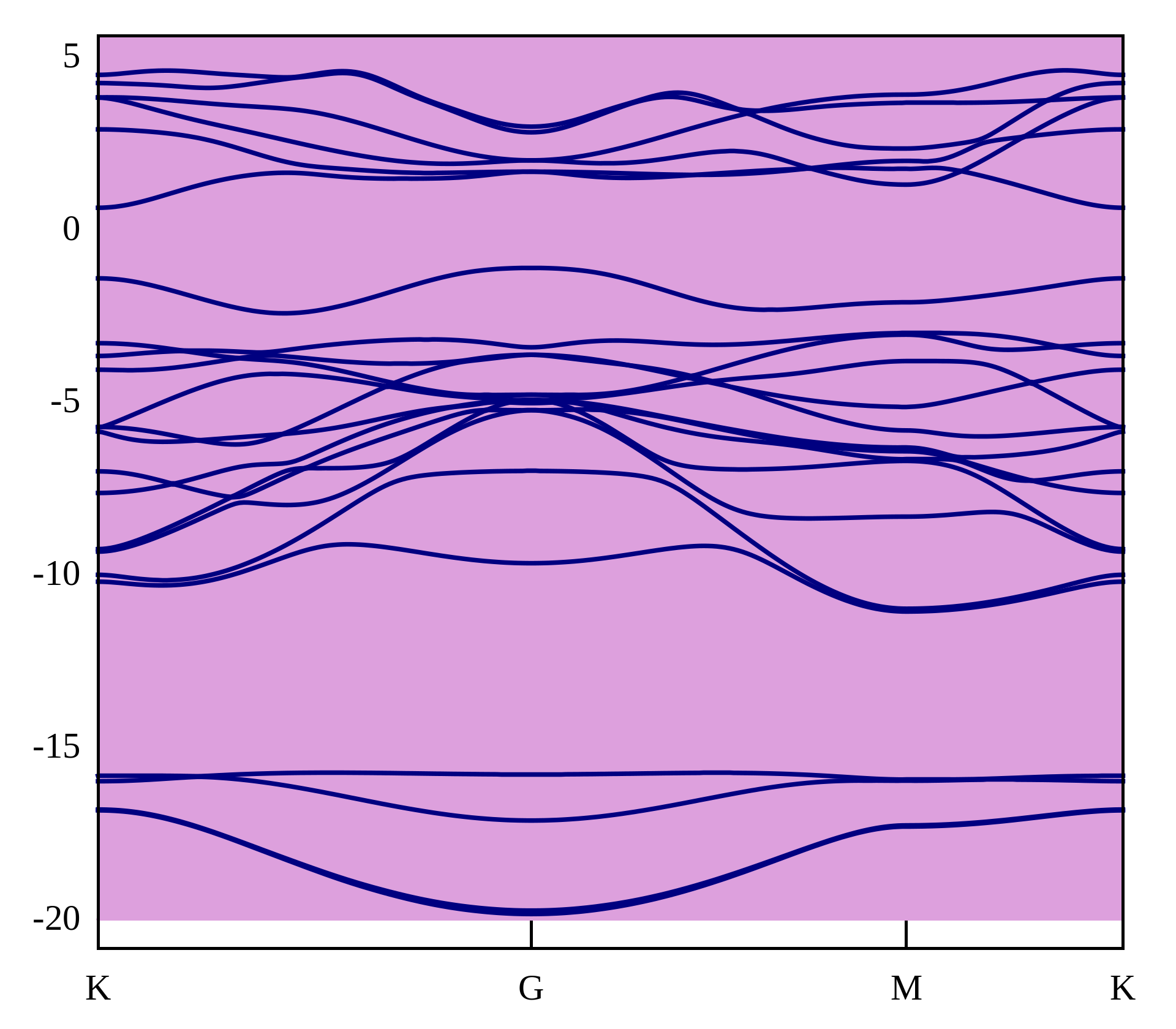
Wannier90 plot
在通过紧束缚模型计算能带的时候,Wannier90虽然会自动给出一个绘制能带的脚本, 但是它并不会保存能带图, 只能立即查看,这是非常不方便的,这里就参考前面的模板来将这个自动产生的脚本进行修改,可执行图片保存,这对后续结果的整理是非常方便的.
set encoding iso_8859_1
set terminal  pngcairo truecolor enhanced lw 5.0 font "TimesNewRoman, 44" size 1920, 1680
#set style data dots
set nokey
set output 'band-wannier90.png'
set xrange [0: 3.40639]
set yrange [-20.85655 :  5.60054]
set arrow from  1.43966, -20.85655 to  1.43966,   5.60054 nohead
set arrow from  2.68656, -20.85655 to  2.68656,   5.60054 nohead
set xtics (" K "  0.00000," G "  1.43966," M "  2.68656," K "  3.40639)
plot -20 with filledcurves y1=20 lc rgb "plum", "wannier90_band.dat" u 1:2 w l lw 1.5 lc rgb "navy"
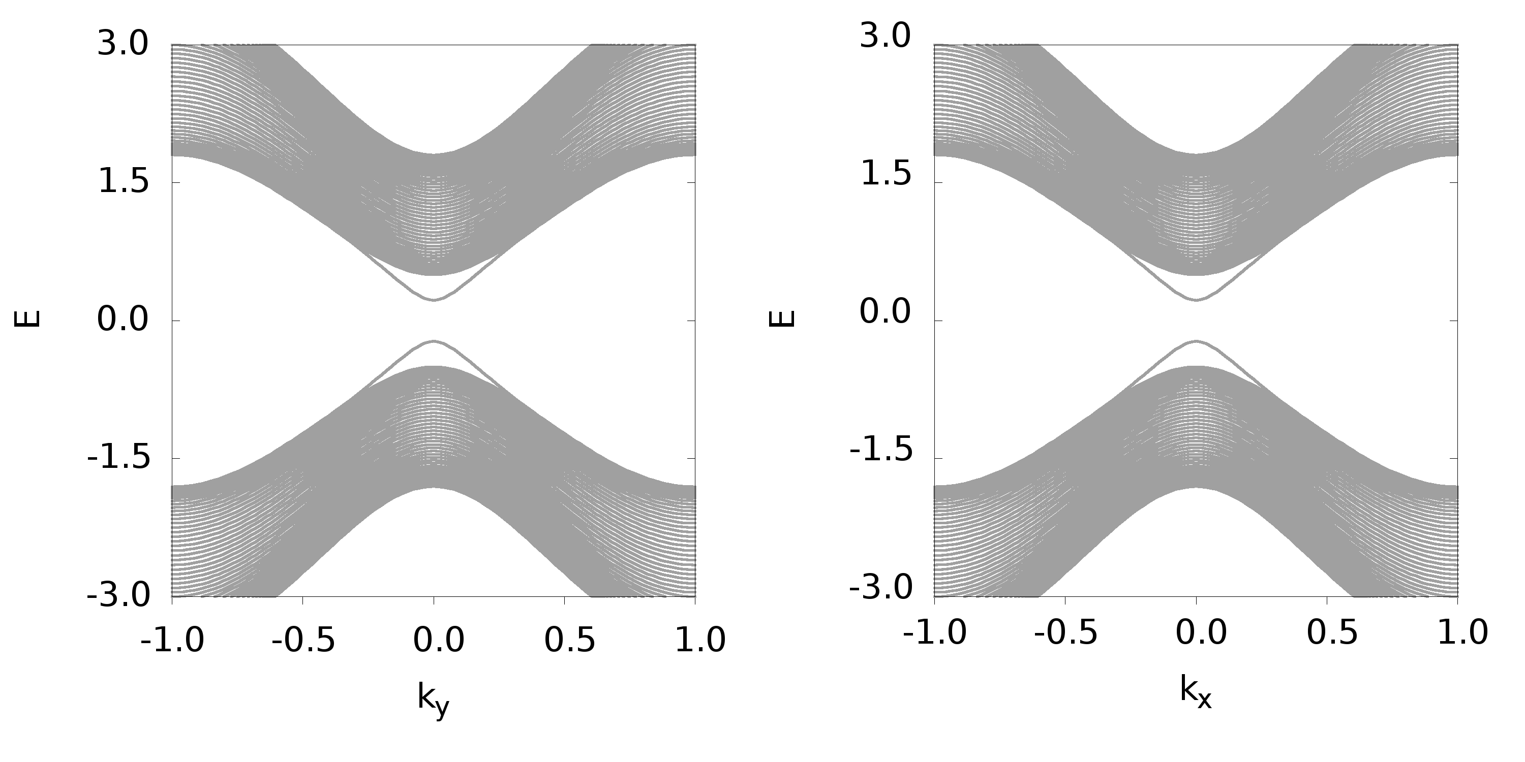
Cylinder 能带图
在计算拓扑边界态的时候通常需要将一个方向开边界,另外一个方向取周期,此时就可以绘制cylinder geometry能带图,绘制代码如下
 set terminal png truecolor enhanced font ",50" size 3000, 1500
 set output 'cy01.png'
 set size 1, 1
 set multiplot layout 1, 2
 unset key
 set ytics 1.5
 set xtics 0.5
 set xtics offset 0, 0.0
 set xtics format "%4.1f" nomirror out
 set ytics format "%4.1f"
 set ylabel "E"
 set ylabel offset 0.5, 0.0
 #set xlabel offset 0, -1.0
 set xrange [-1:1]
 set yrange [-3:3]
 set xlabel 'k_y'
 plot for [i=2:400] 'ox-sc01.dat' u 1:i w l lw 5 lc 'blue'
 set xlabel 'k_x'
 plot for [i=2:400] 'oy-sc01.dat' u 1:i w l lw 5 lc 'blue'
 unset multiplot
结果如下图
产生数据的Fortran程序如下
!   Anticommute mass term
!   tau*spin*orbit
    module pub
    implicit none
    integer yn,kn,ne,N,enn,hn
    real eng   ! energy
    parameter(yn = 50,hn =  8,kn = 50, ne = 50,N = yn*hn)
    real,parameter::pi = 3.1415926535
    complex,parameter::im = (0.,1.0)
    complex Ham(N,N)
    !--------------------------------
    character*12::fn1,fn2,fn3,fn4
    !--------------------------------
    real m0,mu,ax,ay,gamma,tx,ty,dx,dy,d0
    complex g1(hn,hn) ,g4(hn,hn),g2(hn,hn),g3(hn,hn),g5(hn,hn)
    complex am1(hn,hn),am2(hn,hn),am3(hn,hn),am4(hn,hn)
    complex am5(hn,hn),am6(hn,hn),am7(hn,hn),am8(hn,hn),am(hn,hn)
    real mm0,mmx,mmy
    !---------------------------------
    integer::lda = N
    integer,parameter::lwmax = 2*N + N**2
    real,allocatable::w(:)
    complex,allocatable::work(:)
    real,allocatable::rwork(:)
    integer,allocatable::iwork(:)
    integer lwork
    integer lrwork
    integer liwork
    integer info
    end module pub
!================= PROGRAM START ============================
    program sol
    use pub
!====空间申请==================
    allocate(w(N))
    allocate(work(lwmax))
    allocate(rwork(1+5*N+2*N**2))
    allocate(iwork(3+5*N))
!======parameter value setting =====
    m0 = 1.5
    ! mu = 0.3
    tx = 1.0
    ty = 1.0
    ax = 1.0
    ay = 1.0
    ! dx = 0.5
    ! dy = -dx
    mm0 = 0.0
    mmx = 0.5
    mmy = -mmx
    call Pauli()
    ! am = am1
    ! call cylinder()
    call main1()
    ! call plot(1)
    stop
    end program sol
!====================================================================================
    subroutine main1()
    use pub
    am = am1
    call cylinder(1)
    call plot(1)

    am = am2
    call cylinder(2)
    call plot(2)

    am = am3
    call cylinder(3)
    call plot(3)

    am = am5
    call cylinder(5)
    call plot(5)

    am = am6
    call cylinder(6)
    call plot(6)

    am = am7
    call cylinder(7)
    call plot(7)

    am = am8
    call cylinder(8)
    call plot(8)

    end subroutine main1
!=============================================================================================
    subroutine cylinder(m3)
    !  Calculate edge spectrum function
    use pub
    integer m1,m2,m3
    real kx,ky
    character*20::str1,str2,str3,str4,str5,str6
    str1 = "oy-sc"
    str2 = "ox-sc"
    write(str3,"(I2.2)")m3
    str4 = ".dat"
    str5 = trim(str1)//trim(str3)//trim(str4)
    str6 = trim(str2)//trim(str3)//trim(str4)
    open(30,file=str5)
    !-------------------------------------------------
    !   y-direction is open
    do m1 = -kn,kn
        kx = pi*m1/kn
        call openy(kx,0)
        write(30,999)kx/pi,(w(i),i = 1,N)
    end do
    close(30)
    !--------------------------------------------------
    !  x-direction is open
    open(31,file=str6)
    do m1 = -kn,kn
        ky = pi*m1/kn
        call openx(ky,0)
        write(31,999)ky/pi,(w(i),i=1,N)
    end do
    close(31)
999 format(802f11.5)
    return
    end subroutine cylinder
!======================== Pauli Matrix driect product============================
    subroutine Pauli()
    use pub
    !---------Kinetic energy
    g1(1,1) = 1
    g1(2,2) = -1
    g1(3,3) = 1
    g1(4,4) = -1
    g1(5,5) = -1
    g1(6,6) = 1
    g1(7,7) = -1
    g1(8,8) = 1
    !----------SOC-x
    g2(1,2) = 1
    g2(2,1) = 1
    g2(3,4) = -1
    g2(4,3) = -1
    g2(5,6) = 1
    g2(6,5) = 1
    g2(7,8) = -1
    g2(8,7) = -1
    !---------SOC-y
    g3(1,2) = -im
    g3(2,1) = im
    g3(3,4) = -im
    g3(4,3) = im
    g3(5,6) = im
    g3(6,5) = -im
    g3(7,8) = im
    g3(8,7) = -im
    !-------------------SC pairing
    g4(1,7) = -1
    g4(2,8) = -1
    g4(3,5) = 1
    g4(4,6) = 1
    g4(5,3) = 1
    g4(6,4) = 1
    g4(7,1) = -1
    g4(8,2) = -1
    !------------------- Chemical potential
    g5(1,1) = 1
    g5(2,2) = 1
    g5(3,3) = 1
    g5(4,4) = 1
    g5(5,5) = -1
    g5(6,6) = -1
    g5(7,7) = -1
    g5(8,8) = -1
    !-------------------Anti Mass-------------------------------
    !x,y,i TRB
    am1(1,7) = -im
    am1(2,8) = -im
    am1(3,5) = im
    am1(4,6) = im
    am1(5,3) = -im
    am1(6,4) = -im
    am1(7,1) = im
    am1(8,2) = im
    !z,x,x TRB
    am2(1,4) = 1
    am2(2,3) = 1
    am2(3,2) = 1
    am2(4,1) = 1
    am2(5,8) = -1
    am2(6,7) = -1
    am2(7,6) = -1
    am2(8,5) = -1
    !x,x,i TRB
    am3(1,7) = 1
    am3(2,8) = 1
    am3(3,5) = 1
    am3(4,6) = 1
    am3(5,3) = 1
    am3(6,4) = 1
    am3(7,1) = 1
    am3(8,2) = 1
    !y,y,i---> SC Term

    !i,y,x  TRB
    am5(1,4) = -im
    am5(2,3) = -im
    am5(3,2) = im
    am5(4,1) = im
    am5(5,8) = -im
    am5(6,7) = -im
    am5(7,6) = im
    am5(8,5) = im
    !y,x,i  TRS
    am6(1,7) = -im
    am6(2,8) = -im
    am6(3,5) = -im
    am6(4,6) = -im
    am6(5,3) = im
    am6(6,4) = im
    am6(7,1) = im
    am6(8,2) = im
    !i,x,x TRB
    am7(1,4) = 1
    am7(2,3) = 1
    am7(3,2) = 1
    am7(4,1) = 1
    am7(5,8) = 1
    am7(6,7) = 1
    am7(7,6) = 1
    am7(8,5) = 1
    !z,x,y TRB
    am8(1,4) = -im
    am8(2,3) = im
    am8(3,2) = -im
    am8(4,1) = im
    am8(5,8) = im
    am8(6,7) = -im
    am8(7,6) = im
    am8(8,5) = -im
    return
    end subroutine Pauli
!==========================================================
    subroutine openx(ky,input)
    use pub
    real ky
    integer m,l,k,input
    Ham = 0
!========== Positive energy ========
    do k = 0,yn-1
        if (k == 0) then ! Only right block in first line
            do m = 1,hn
                do l = 1,hn
                    Ham(m,l) = (m0-ty*cos(ky))*g1(m,l) + ay*sin(ky)*g3(m,l) + (d0 + dy*cos(ky))*g4(m,l)
                    Ham(m,l) = Ham(m,l) + (mm0 + mmy*cos(ky))*am(m,l)

                    Ham(m,l + hn) = (-tx*g1(m,l) - im*ax*g2(m,l) - im*del*g4(m,l))/2 + dx/2.0*g4(m,l)
                    Ham(m,l + hn) = Ham(m,l + hn) + mmx/2.0*am(m,l)
                end do
            end do
        elseif ( k==yn-1 ) then ! Only left block in last line
            do m = 1,hn
                do l = 1,hn
                    Ham(k*hn + m,k*hn + l) = (m0-ty*cos(ky))*g1(m,l) + ay*sin(ky)*g3(m,l) + (d0 + dy*cos(ky))*g4(m,l)
                    Ham(k*hn + m,k*hn + l) = Ham(k*hn + m,k*hn + l) + (mm0 + mmy*cos(ky))*am(m,l)

                    Ham(k*hn + m,k*hn + l - hn) = -tx*g1(m,l)/2 + im*ax*g2(m,l)/2 + im*del*g4(m,l)/2.0 + dx/2.0*g4(m,l)
                    Ham(k*hn + m,k*hn + l - hn) = Ham(k*hn + m,k*hn + l - hn) + mmx/2.0*am(m,l)
                end do
            end do
        else
            do m = 1,hn
                do l = 1,hn ! k start from 1,matrix block from 2th row
                    Ham(k*hn + m,k*hn + l) = (m0 - ty*cos(ky))*g1(m,l) + ay*sin(ky)*g3(m,l) + (d0 + dy*cos(ky))*g4(m,l)
                    Ham(k*hn + m,k*hn + l) = Ham(k*hn + m,k*hn + l) + (mm0 + mmy*cos(ky))*am(m,l)

                    Ham(k*hn + m,k*hn + l + hn) = (-tx*g1(m,l) - im*ax*g2(m,l))/2 + dx/2.0*g4(m,l)
                    Ham(k*hn + m,k*hn + l + hn) = Ham(k*hn + m,k*hn + l + hn) + mmx/2.0*am(m,l)

                    Ham(k*hn + m,k*hn + l - hn) = -tx*g1(m,l)/2 + im*ax*g2(m,l)/2 + dx/2.0*g4(m,l)
                    Ham(k*hn + m,k*hn + l - hn) = Ham(k*hn + m,k*hn + l - hn) + mmx/2.0*am(m,l)
                end do
            end do
        end if
    end do
    !------------------------
    call isHermitian()
    call eigsol(input)
    return
    end subroutine openx
!==========================================================
    subroutine openy(kx,input)
    use pub
    real kx
    integer m,l,k,input
    Ham = 0
!========== Positive energy ========
    do k = 0,yn-1
        if (k == 0) then ! Only right block in first line
            do m = 1,hn
                do l = 1,hn
                    Ham(m,l) = (m0-tx*cos(kx))*g1(m,l) + ax*sin(kx)*g2(m,l) + (d0 + dx*cos(kx))*g4(m,l)
                    Ham(m,l) = Ham(m,l) + (mm0 + mmx*cos(kx))*am(m,l)

                    Ham(m,l + hn) = (-ty*g1(m,l) - im*ay*g3(m,l))/2 + dy/2.0*g4(m,l)
                    Ham(m,l + hn) = Ham(m,l + hn) + mmy/2.0*am(m,l)
                end do
            end do
        elseif ( k==yn-1 ) then ! Only left block in last line
            do m = 1,hn
                do l = 1,hn
                    Ham(k*hn + m,k*hn + l) = (m0-tx*cos(kx))*g1(m,l) + ax*sin(kx)*g2(m,l) + (d0 + dx*cos(kx))*g4(m,l)
                    Ham(k*hn + m,k*hn + l) = Ham(k*hn + m,k*hn + l) + (mm0 + mmx*cos(kx))*am(m,l)

                    Ham(k*hn + m,k*hn + l - hn) = -ty*g1(m,l)/2 + im*ay*g3(m,l)/2 + dy/2.0*g4(m,l)
                    Ham(k*hn + m,k*hn + l - hn) = Ham(k*hn + m,k*hn + l - hn) + mmy/2.0*am(m,l)
                end do
            end do
        else
            do m = 1,hn
                do l = 1,hn ! k start from 1,matrix block from 2th row
                    Ham(k*hn + m,k*hn + l) = (m0-tx*cos(kx))*g1(m,l) + ax*sin(kx)*g2(m,l) + (d0 + dx*cos(kx))*g4(m,l)
                    Ham(k*hn + m,k*hn + l) = Ham(k*hn + m,k*hn + l) + (mm0 + mmx*cos(kx))*am(m,l)

                    Ham(k*hn + m,k*hn + l + hn) = (-ty*g1(m,l) - im*ay*g3(m,l) )/2 + dy/2.0*g4(m,l)
                    Ham(k*hn + m,k*hn + l + hn) = Ham(k*hn + m,k*hn + l + hn) + mmy/2.0*am(m,l)

                    Ham(k*hn + m,k*hn + l - hn) = -ty*g1(m,l)/2 + im*ay*g3(m,l)/2 + dy/2.0*g4(m,l)
                    Ham(k*hn + m,k*hn + l - hn) = Ham(k*hn + m,k*hn + l - hn) + mmy/2.0*am(m,l)
                end do
            end do
        end if
    end do
    !---------------------------------
    call isHermitian()
    call eigsol(input)
    return
    end subroutine openy
!============================================================
    subroutine isHermitian()
    use pub
    integer i,j
    do i = 1,N
        do j = 1,N
            if (Ham(i,j) .ne. conjg(Ham(j,i)))then
                open(160,file = 'hermitian.dat')
                write(160,*)i,j
                write(160,*)Ham(i,j)
                write(160,*)Ham(j,i)
                write(160,*)"===================="
                write(*,*)"Hamiltonian is not hermitian"
                stop
            end if
        end do
    end do
    close(160)
    return
    end subroutine isHermitian
!================= Hermitain Matrices solve ==============
    subroutine eigsol(input)
    use pub
    integer m
    character*20::str1,str2,str3,str4
    str1 = "eigval"
    str3 = ".dat"
    write(str2,"(I4.4)")input
    str4 = trim(str1)//trim(str2)//trim(str3)
    lwork = -1
    liwork = -1
    lrwork = -1
    call cheevd('V','U',N,Ham,lda,w,work,lwork,rwork,lrwork,iwork,liwork,info)
    lwork = min(2*N+N**2, int( work( 1 ) ) )
    lrwork = min(1+5*N+2*N**2, int( rwork( 1 ) ) )
    liwork = min(3+5*N, iwork( 1 ) )
    call cheevd('V','U',N,Ham,lda,w,work,lwork,rwork,lrwork,iwork,liwork,info)
    if( info .GT. 0 ) then
        open(110,file="mes.dat",status="unknown")
        write(110,*)'The algorithm failed to compute eigenvalues.'
        close(110)
    end if
    return
    end subroutine eigsol
!==========================================================================
    subroutine plot(m3)
    use pub
    character*20::str1,str2,str3,str4,str5,str6
    integer m3
    str1 = "half"
    write(str2,"(I2.2)")m3
    str3 = ".gnu"
    str4 = trim(str1)//trim(str2)//trim(str3)
    open(20,file=str4)
    write(20,*)'set terminal png truecolor enhanced font ",50" size 3000, 1500'
    write(20,*)"set output 'cy"//trim(str2)//".png'"
    write(20,*)"set size 1, 1"
    write(20,*)"set multiplot layout 1, 2"
    write(20,*)"unset key"
    write(20,*)"set ytics 1.5 "
    write(20,*)"set xtics 0.5"
    write(20,*)"set xtics offset 0, 0.0"
    write(20,*)'set xtics format "%4.1f" nomirror out '
    write(20,*)'set ytics format "%4.1f"'
    write(20,*)'set ylabel "E"'
    write(20,*)"set ylabel offset 0.5, 0.0 "
    write(20,*)"#set xlabel offset 0, -1.0 "
    write(20,*)"set xrange [-1:1]"
    write(20,*)"set yrange [-3:3]"
    write(20,*)"set xlabel 'k_y' "
    write(20,*)"plot for [i=2:400] 'ox-sc"//trim(str2)//".dat' u 1:i w l lw 5 lc 'blue'"
    write(20,*)"set xlabel 'k_x' "
    write(20,*)"plot for [i=2:400] 'oy-sc"//trim(str2)//".dat' u 1:i w l lw 5 lc 'blue'"
    write(20,*)"unset multiplot"
    close(20)
    end subroutine plot
这个程序可以产生一系列的绘图文件.gnu**以及绘图数据.dat**,可以通过一个shell脚本来批量执行
#!/bin/sh
#============ get the file name ===========
Folder_A=$(pwd)
for file_a in ${Folder_A}/*.gnu
do
	gnuplot $file_a
done
这个脚本可以执行这个当前文件夹下面所有的.gnu文件。
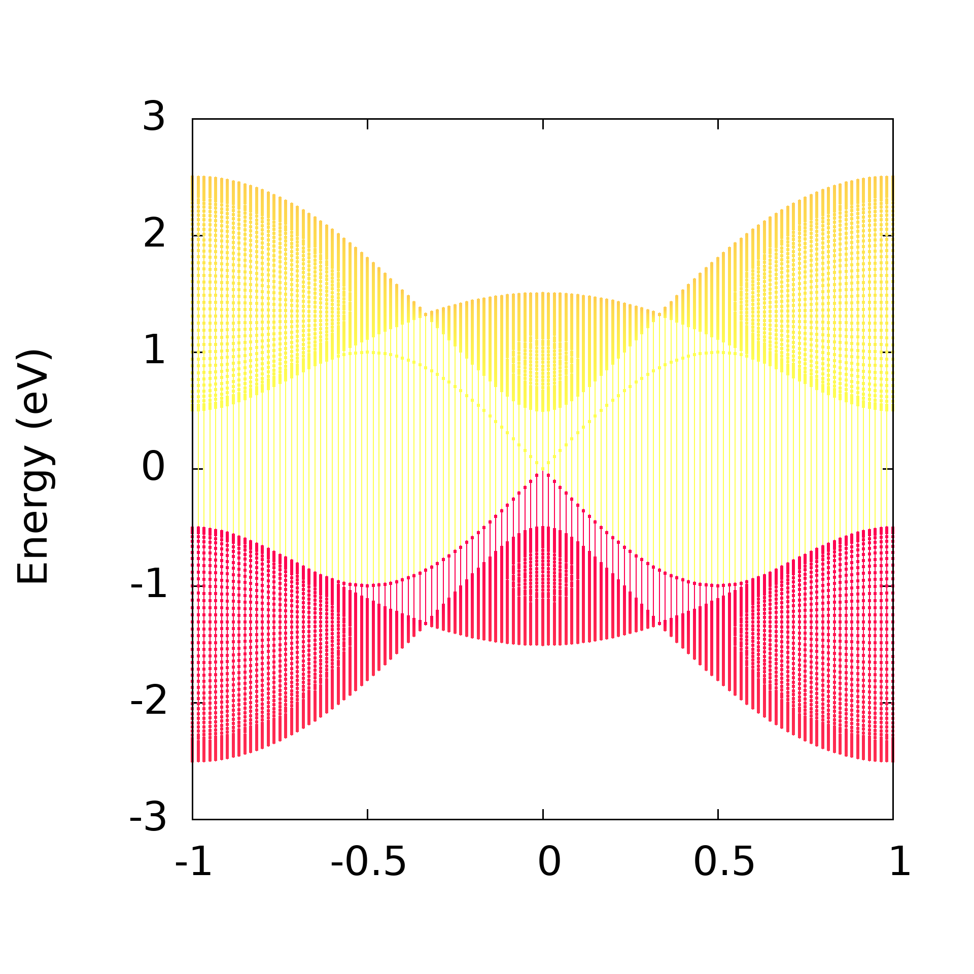
线条权重染色
set encoding iso_8859_1
#set terminal  postscript enhanced color
#set output 'c1.eps'
#set terminal  pngcairo truecolor enhanced  font ",60" size 1920, 1680
set terminal  png truecolor enhanced  font ",60" size 1920, 1920
set output 'c1.png'
set palette defined ( 0  "green", 5 "yellow", 10 "red" )
set style data linespoints
unset ztics
unset key
set pointsize 0.8
set border lw 3
set view 0,0
#set xtics font ",36"
#set ytics font ",36"
#set ylabel font ",36"
set size ratio 1
#set xtics offset 0, -1
set ylabel offset -1, 0
set xrange [-1:1]
set ylabel "Energy (eV)"
set yrange [-3:3]
rgb(r,g,b) = int(r)*65536 + int(g)*256 + int(b)
plot 'c1.dat' u 1:2:(rgb(255,$3, 80)) w lp lw 2 pt 7  ps 1 lc rgb variable # RGB颜色绘图
# (a)
# plot the top and bottom surface's weight together
#plot 'c1.dat' u 1:2:($3+$4) w lp lw 2 pt 7  ps 1 lc palette
# (b)
# plot top and bottom surface's weight with red and blue respectively
set palette defined ( -1  "green",-0.0001 "red" , 0 "blue", 0.00001 "red", 1 "red" )
#plot 'c1.dat' u 1:2:($4-$3) w lp lw 5  lc palette
#plot 'c1.dat' u 1:2 w lp lw 5  lc 'blue'
产生数据的代码如下
!   Author: YuXuanLi
!   Email:yxli406@gmail.com
    module pub
    implicit none
    integer yn,kn,hnn
    parameter(yn = 50,kn = 60,hnn = 2)
    integer,parameter::N = yn*hnn
    real,parameter::pi = 3.1415926535
    complex,parameter::im = (0.,1.0)
    complex::Ham(N,N) = 0
    complex g1(hnn,hnn),g2(hnn,hnn),g3(hnn,hnn)
    real m0,tx,ty,lamx,lamy
    !--------------------------------------
    integer::lda = N
    integer,parameter::lwmax=2*N+N**2
    real,allocatable::w(:)
    complex,allocatable::work(:)
    real,allocatable::rwork(:)
    integer,allocatable::iwork(:)
    integer lwork
    integer lrwork
    integer liwork
    integer info
    end module pub
!============================================================
    program sol
    use pub
    allocate(w(N))
    allocate(work(lwmax))
    allocate(rwork(1+5*N+2*N**2))
    allocate(iwork(3+5*N))
    !------------------------------------
    m0 = 0.5
    tx = 1.0
    ty = -1.0
    lamx = 1.0
    lamy = 1.0
    ! call main1()
    call main2()
    call plot()
    stop
    end program sol
!============================================================
    subroutine main1()
    use pub
    integer m1
    real k
    open(3,file="openx-m1.dat")
    open(4,file="openy-m1.dat")
    do m1 = -kn,kn
        k = pi*m1/kn
        call openx(k)
        write(3,999)k/pi,(w(i),i = 1,N)
        call openy(k)
        write(4,999)k/pi,(w(i),i = 1,N)
    end do
    close(3)
    close(4)
999 format(201f11.6)
    end subroutine main1
!============================================================
    subroutine main2()
    use pub
    integer m1,m2
    real k
    open(3,file="c1.dat")
    open(4,file="c2.dat")
    ! write(3,*)"kx","E","W1","W2"
    ! write(4,*)"kx","E","W1","W2"
    do m1 = -kn,kn
        k = pi*m1/kn
        call openx(k)
        do m2 = 1,N
            ! write(3,*)k/pi,w(m2),sin(1.0*(N/2-m2)),cos(1.0*m2)
            write(3,*)k/pi,w(m2),N/2-m2,m2
        end do
        write(3,*)" "
        call openy(k)
        do m2 = 1,N
            ! write(4,*)k/pi,w(m2),sin(1.0*(N/2-m2)),cos(1.0*m2)
            write(4,*)k/pi,w(m2),N/2-m2,m2
        end do
        write(4,*)" "
    end do
    close(3)
    close(4)
    end subroutine main2
!============================================================
    subroutine openx(ky)
    use pub
    real ky
    call pauli()
    Ham = 0
    !========== Positive energy ========
    do k = 0,yn-1
        if (k == 0) then ! Only right block in first line
            do m = 1,hnn
                do l = 1,hnn
                    Ham(m,l) = lamy*sin(ky)*g2(m,l) + (m0 + ty*cos(ky))*g3(m,l)

                    Ham(m,l + hnn) = tx/2.0*g3(m,l) + lamx/(2*im)*g1(m,l)
                end do
            end do
        elseif ( k==yn-1 ) then ! Only left block in last line
            do m = 1,hnn
                do l = 1,hnn
                    Ham(k*hnn + m,k*hnn + l) = lamy*sin(ky)*g2(m,l) + (m0 + ty*cos(ky))*g3(m,l)

                    Ham(k*hnn + m,k*hnn + l - hnn) = tx/2.0*g3(m,l) - lamx/(2*im)*g1(m,l)
                end do
            end do
        else
            do m = 1,hnn
                do l = 1,hnn ! k start from 1,matrix block from 2th row
                    Ham(k*hnn + m,k*hnn + l) = lamy*sin(ky)*g2(m,l) + (m0 + ty*cos(ky))*g3(m,l)

                    Ham(k*hnn + m,k*hnn + l + hnn) = tx/2.0*g3(m,l) + lamx/(2*im)*g1(m,l)
                    Ham(k*hnn + m,k*hnn + l - hnn) = tx/2.0*g3(m,l) - lamx/(2*im)*g1(m,l)
                end do
            end do
        end if
    end do
    !------------------------
    call isHermitian()
    call eigsol()
    return
    end subroutine openx
!============================================================
    subroutine openy(kx)
    use pub
    real kx
    call pauli()
    Ham = 0
    !========== Positive energy ========
    do k = 0,yn-1
        if (k == 0) then ! Only right block in first line
            do m = 1,hnn
                do l = 1,hnn
                    Ham(m,l) = lamx*sin(kx)*g1(m,l) + (m0 + tx*cos(kx))*g3(m,l)

                    Ham(m,l + hnn) = lamy/(2*im)*g2(m,l) + ty/2.0*g3(m,l)
                end do
            end do
        elseif ( k==yn-1 ) then ! Only left block in last line
            do m = 1,hnn
                do l = 1,hnn
                    Ham(k*hnn + m,k*hnn + l) = lamx*sin(kx)*g1(m,l) + (m0 + tx*cos(kx))*g3(m,l)

                    Ham(k*hnn + m,k*hnn + l - hnn) = -lamy/(2*im)*g2(m,l) + ty/2.0*g3(m,l)
                end do
            end do
        else
            do m = 1,hnn
                do l = 1,hnn ! k start from 1,matrix block from 2th row
                    Ham(k*hnn + m,k*hnn + l) = lamx*sin(kx)*g1(m,l) + (m0 + tx*cos(kx))*g3(m,l)

                    Ham(k*hnn + m,k*hnn + l + hnn) = lamy/(2*im)*g2(m,l) + ty/2.0*g3(m,l)
                    Ham(k*hnn + m,k*hnn + l - hnn) = -lamy/(2*im)*g2(m,l) + ty/2.0*g3(m,l)
                end do
            end do
        end if
    end do
    !------------------------
    call isHermitian()
    call eigsol()
    return
    end subroutine openy
!============================================================
    subroutine pauli()
    use pub
    g1(1,hnn) = 1
    g1(2,1) = 1
    !-----------------
    g2(1,hnn) = -im
    g2(2,1) = im
    !---------------
    g3(1,1) = 1
    g3(2,2) = -1
    end subroutine pauli
!============================================================
    subroutine isHermitian()
    use pub
    integer i,j
    do i = 1,N
        do j = 1,N
            if (Ham(i,j) .ne. conjg(Ham(j,i)))then
                open(16,file = 'hermitian.dat')
                write(16,*)i,j
                write(16,*)Ham(i,j)
                write(16,*)Ham(j,i)
                write(16,*)"===================="
                write(*,*)"Ham isn't Hermitian"
                stop
            end if
        end do
    end do
    close(16)
    return
    end subroutine isHermitian
!================= 矩阵本征值求解 ==============
    subroutine eigSol()
    use pub
    integer m
    lwork = -1
    liwork = -1
    lrwork = -1
    call cheevd('V','Upper',N,Ham,lda,w,work,lwork &
        ,rwork,lrwork,iwork,liwork,info)
    lwork = min(2*N+N**2, int( work( 1 ) ) )
    lrwork = min(1+5*N+2*N**2, int( rwork( 1 ) ) )
    liwork = min(3+5*N, iwork( 1 ) )
    call cheevd('V','Upper',N,Ham,lda,w,work,lwork &
        ,rwork,lrwork,iwork,liwork,info)
    if( info .GT. 0 ) then
        open(11,file="mes.dat",status="unknown")
        write(11,*)'The algorithm failed to compute eigenvalues.'
        close(11)
    end if
    return
    end subroutine eigSol
!=====================================================================
    subroutine plot()
    use pub
    open(20,file="plot.gnu")
    write(20,111)"set encoding iso_8859_1"
    write(20,111)"#set terminal  postscript enhanced color"
    write(20,111)"#set output 'c1.eps'"
    write(20,111)'#set terminal  pngcairo truecolor enhanced  font ",60" size 1920, 1680'
    write(20,111)'set terminal  png truecolor enhanced  font ",60" size 1920, 1920'
    write(20,111)"set output 'c1.png'"
    write(20,111)'set palette defined ( 0  "green", 5 "yellow", 10 "red" )'
    write(20,111)"set style data linespoints"
    write(20,111)"unset ztics"
    write(20,111)"unset key"
    write(20,111)"set pointsize 0.8"
    write(20,111)"set border lw 3 "
    write(20,111)"set view 0,0"
    write(20,111)'#set xtics font ",36"'
    write(20,111)'#set ytics font ",36"'
    write(20,111)'#set ylabel font ",36"'
    write(20,111)'set size ratio 1'
    write(20,111)"#set xtics offset 0, -1"
    write(20,111)"set ylabel offset -1, 0 "
    write(20,111)"set xrange [-1:1]"
    write(20,111)'set ylabel "Energy (eV)"'
    write(20,111)"set yrange [-3:3]"
    write(20,111)"rgb(r,g,b) = int(r)*65536 + int(g)*256 + int(b)"
    write(20,111)"plot 'c1.dat' u 1:2:(rgb(255,$3, 3)) w lp lw 2 pt 7  ps 1 lc rgb variable"
    write(20,111)"# (a) "
    write(20,111)"# plot the top and bottom surface's weight together"
    write(20,111)"#plot 'c1.dat' u 1:2:($3+$4) w lp lw 2 pt 7  ps 1 lc palette"
    write(20,111)"# (b) "
    write(20,111)"# plot top and bottom surface's weight with red and blue respectively"
    write(20,111)'set palette defined ( -1  "green",-0.0001 "red" , 0 "blue", 0.00001 "red", 1 "red" )'
    write(20,111)"#plot 'c1.dat' u 1:2:($4-$3) w lp lw 5  lc palette"
    write(20,111)"#plot 'c1.dat' u 1:2 w lp lw 5  lc 'blue'"
    close(20)
111 format(A85)
    return
    end subroutine plot
上面fortran程序可以通过ifort -mkl filename.f90进行编译执行.产生的gnuplot绘图文件也可以通过上一节的绘图脚本来执行.
绘制两条曲线做对比
# 绘制VASP计算能带图与Wannier90拟合能带图
set style data dots
set encoding iso_8859_1
set terminal png truecolor enhanced font ",50" size 1920, 1680
set size 0.9,1
set output 'wannier90_band.png'
#set nokey
set key font "Times,24,Bold"
set key Right at 5,5
set xrange [0: 4.27065]
set yrange [-5 : 5]
#set arrow from  0.84341,  -6.29553 to  0.84341,  14.22923 nohead
#set arrow from  2.46594,  -6.29553 to  2.46594,  14.22923 nohead
#set arrow from  3.42724,  -6.29553 to  3.42724,  14.22923 nohead
#set ytics offset -1,0 font 'Times,Bold'
#set xtics offset 0,-0.1 font 'Times,Bold'
set ytics font 'Times,Bold'
set xtics font 'Times,Bold'
set xtics ("G"  0.00000,"Z"  0.84341,"F"  2.46594,"G"  3.42724,"L"  4.27065)
#plot "wannier90_band.dat" w p  pt 7  ps 1.1 lc 'red',"BAND.dat" w p pt 7 ps 1.1 lc 'blue'
plot "wannier90_band.dat" w l  lw 5.0 lt 7 lc 'red' title "wannier","BAND.dat" w l lw 5.0 lt 7  lc 'blue' title "VASP"
这里需要使用VASP计算得到的能带数据和wannier90得到的能带数据来一起绘制,这么做也是为了比较做wannier的时候,做的到底好不好,通常情况下二者在费米面附近应该是要拟合的非常好才可以认为是wannier化比较成功。
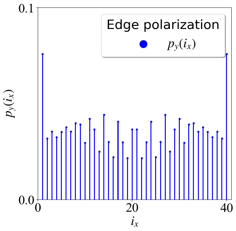
棒棒糖图
from cProfile import label
from turtle import color
import numpy as np
import matplotlib.pyplot as plt
from matplotlib import rcParams
import os
config = {
"font.size": 30,
"mathtext.fontset":'stix',
"font.serif": ['SimSun'],
}
rcParams.update(config) # Latex 字体设置
#---------------------------------------------------------
def scatter1(cont):
    #da1 = "m" + str(cont) + "-pro-ox"  + ".dat"
    #da2 = "m" + str(cont) + "-pro-oy"  + ".dat"
    da1 = "rho-mu-ix.dat"
    picname = "rho-ix-" + str(cont) + ".png"
    os.chdir(os.getcwd())# 确定用户执行路径
    x0 = []
    y0 = []
    with open(da1) as file:
        da = file.readlines()
        for f1 in da:
            if len(f1) > 3:
                ldos = [float(x) for x in f1.strip().split()]
                x0.append(ldos[0])
                y0.append(ldos[cont]) # 这里是有多列数据才这样操作的
    y0 = np.array(y0)
    plt.figure(figsize=(8,8))
    plt.bar(x0,y0,width=0.2,color='blue')
    # plt.scatter(x0, y0, s = 20, color = 'blue', alpha = 0.7, linewidths = 0.3,label = "$p_y(i_x)$")
    plt.scatter(x0, y0, s = 20, color = 'blue',  linewidths = 0.3,label = "$p_y(i_x)$")
    # plt.plot(x0, y0, c = 'blue', alpha = 0.5, markersize = 6,marker = 'o',label = "$p_y(i_x)$")
    #plt.legend("x0")
    x0min = np.min(x0)
    x0max = np.max(x0)
    font2 = {'family': 'Times New Roman',
             'weight': 'normal',
             'size': 30,
             }
    plt.xlim(x0min,x0max+1)
    #plt.legend("x1")
    # plt.ylim(-0.01,0.13)
    plt.xlabel("$i_x$",font2)
    plt.ylabel("$p_y(i_x)$",font2)
    plt.legend(loc = 'upper right', ncol = 2, title = 'Edge polarization', shadow = True, fancybox = True, prop = font2,markerscale = 4)
    plt.xticks([0,20,40],fontproperties='Times New Roman', size = 30)
    plt.yticks([0,0.1],fontproperties='Times New Roman', size = 30)
    plt.savefig(picname, dpi = 100, bbox_inches = 'tight')
    plt.close()
#---------------------------------------------------------
def scatter2(cont):
    #da1 = "m" + str(cont) + "-pro-ox"  + ".dat"
    #da2 = "m" + str(cont) + "-pro-oy"  + ".dat"
    da2 = "rho-mu-iy.dat"
    picname = "rho-iy-" + str(cont) + ".png"
    os.chdir(os.getcwd())# 确定用户执行路径
    x0 = []
    y0 = []
    x1 = []
    y1 = []
    with open(da2) as file:
        da = file.readlines()
        for f1 in da:
            if len(f1) > 3:
                ldos = [float(x) for x in f1.strip().split()]
                x1.append(ldos[0])
                y1.append(ldos[cont])
    y1 = np.array(y1)
    plt.figure(figsize=(8,8))
    # sc = plt.scatter(x0, y0, c = z1, s = 2,vmin = 0, vmax = 1, cmap="magma")
    # plt.plot(x1, y1, c = 'red', alpha = 0.7, markersize = 6,marker = 'o',label = "$p_x(i_y)$")
    plt.bar(x1,y1,width=0.2,color='red')
    # plt.scatter(x1, y1, s = 20, color = 'red', alpha = 0.7, linewidths = 0.3,label = "$p_x(i_y)$")
    plt.scatter(x1, y1, s = 20, color = 'red',linewidths = 0.3,label = "$p_x(i_y)$")
    x0min = np.min(x1)
    x0max = np.max(x1)
    font2 = {'family': 'Times New Roman',
             'weight': 'normal',
             'size': 30,
             }
    plt.xlim(x0min,x0max+1)
    #plt.legend("x1")
    # plt.ylim(-0.01,0.13)
    plt.xlabel("$i_y$",font2)
    plt.ylabel("$p_x(i_y)$",font2)
    plt.legend(loc = 'upper right', ncol = 2, title = 'Edge polarization', shadow = True, fancybox = True, prop = font2,markerscale = 4)
    plt.xticks([0,20,40],fontproperties='Times New Roman', size = 30)
    plt.yticks([0,0.1],fontproperties='Times New Roman', size = 30)
    plt.savefig(picname, dpi = 100, bbox_inches = 'tight')
    plt.close()
#---------------------------------------------------------
def main():
    for i0 in range(1,50):
        scatter1(i0)
        scatter2(i0)
#---------------------------------------------------------
if __name__=="__main__":
    main()
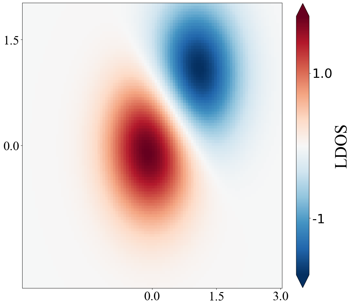
密度图(Python)
def density():
    os.chdir(os.getcwd())# 确定用户执行路径
    picname = "density.png"
    N = 100
    X, Y = np.mgrid[-3:3:complex(0, N), -2:2:complex(0, N)] # 这里步长是复数,表示以点数来进行分割
    Z1 = np.exp(-X**2 - Y**2)
    Z2 = np.exp(-(X - 1)**2 - (Y - 1)**2)
    Z = (Z1 - Z2) * 2
    plt.figure(figsize=(12,12))
    fig = plt.pcolormesh(X, Y, Z, cmap='RdBu_r', vmin=np.min(Z),shading='nearest')
    # fig = plt.pcolormesh(X, Y, Z, cmap='RdBu_r', vmin = -1, vmax = 1,shading='nearest')
    cb = plt.colorbar(fig,fraction = 0.045,extend = 'both')  # 调整colorbar的大小和图之间的间距
    cb.ax.tick_params(labelsize=30) # corbar标签大小
    cb.set_ticks(np.linspace(-1,1,2)) # color 刻度设置
    cb.set_ticklabels(('-1','1.0'))
    font2 = {'family': 'Times New Roman',
             'weight': 'normal',
             'size': 40,
             }
    cb.set_label('LDOS',fontdict = font2) #设置colorbar的标签字体及其大小
    # plt.axis('scaled')
    plt.yticks([0,1.5],fontproperties='Times New Roman', size = 30)
    plt.xticks([0,1.5,3],fontproperties='Times New Roman', size = 30)
    plt.savefig(picname, dpi=100,bbox_inches = 'tight')
    plt.show()
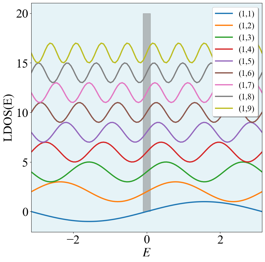
y轴堆叠图
import matplotlib.pyplot as plt
import numpy as np
import os
from matplotlib import rcParams
config = {"font.size": 30,"mathtext.fontset":'stix',"font.serif": ['SimSun']}
rcParams.update(config) # Latex 字体设置
#-----------------------------------------------------
def plot1(cont):
    # y轴平移堆叠图
    # da1 = "ldos-" + str(cont).rjust(4,'0') + ".dat"
    da1 = "h0-ldos-v2.dat"
    picname = "ldos-" + str(cont).rjust(4,'0') + ".png"
    os.chdir(os.getcwd())# 确定用户执行路径
    x0 = np.linspace(-np.pi,np.pi,100)
    plt.figure(figsize=(10,10))
    for i0 in range(1,10):
        lab = "(1," + str(i0) + ")"
        plt.plot(x0,np.sin(i0*x0) + (i0 - 1)*2,label = lab,lw = 3.0)
    x0min = np.min(x0)
    x0max = np.max(x0)
    font2 = {'family': 'Times New Roman','weight': 'normal','size': 30,}
    font1 = {'family': 'Times New Roman','weight': 'normal','size': 20,}
    # plt.xlim(x0min,x0max)
    plt.xlim(x0min,x0max)
    # plt.ylim(y0min,y0max + 1)
    # plt.ylim(-0.5,0.5)
    plt.xlabel(r'$E$',font2)
    plt.ylabel("LDOS(E)",font2)
    plt.yticks(fontproperties='Times New Roman', size = 30)
    plt.xticks(fontproperties='Times New Roman', size = 30)
    #plt.xticks([-1,-0.75,0,0.75,1],fontproperties='Times New Roman', size = 20)
    #plt.yticks([-0.5,0,0.5],fontproperties='Times New Roman', size = 20)
    #plt.vlines(x = 0.75, ymin = -1, ymax = 1,lw = 3.0, colors = 'blue', linestyles = '--')
    #plt.vlines(x = -0.75, ymin = -1, ymax = 1,lw = 3.0, colors = 'blue', linestyles = '--')
    wid = 0.1
    x = [-wid,wid,wid,-wid]
    y = [0,0,20,20]
    plt.fill(x,y,c = "gray",alpha = 0.5) # 颜色填充
    # plt.legend(prop = font2)
    plt.legend(loc='upper right', shadow=True, fancybox=True,prop = font1)
    ax1=plt.gca()
    ax1.patch.set_facecolor("lightblue")    # 设置 ax1 区域背景颜⾊
    ax1.patch.set_alpha(0.3)    # 设置 ax1 区域背景颜⾊透明度
    plt.savefig(picname, dpi = 100, bbox_inches = 'tight')
    plt.show()
#-------------------------------------------------------------------
plot1(1)
for i0 in range(1,10):
        lab = "(1," + str(i0) + ")"
        plt.plot(x0,np.sin(i0*x0) + (i0 - 1)*2,label = lab,lw = 3.0)
这里只需要把 (i0 - 1)*2去掉就可以实现非堆叠的效果。
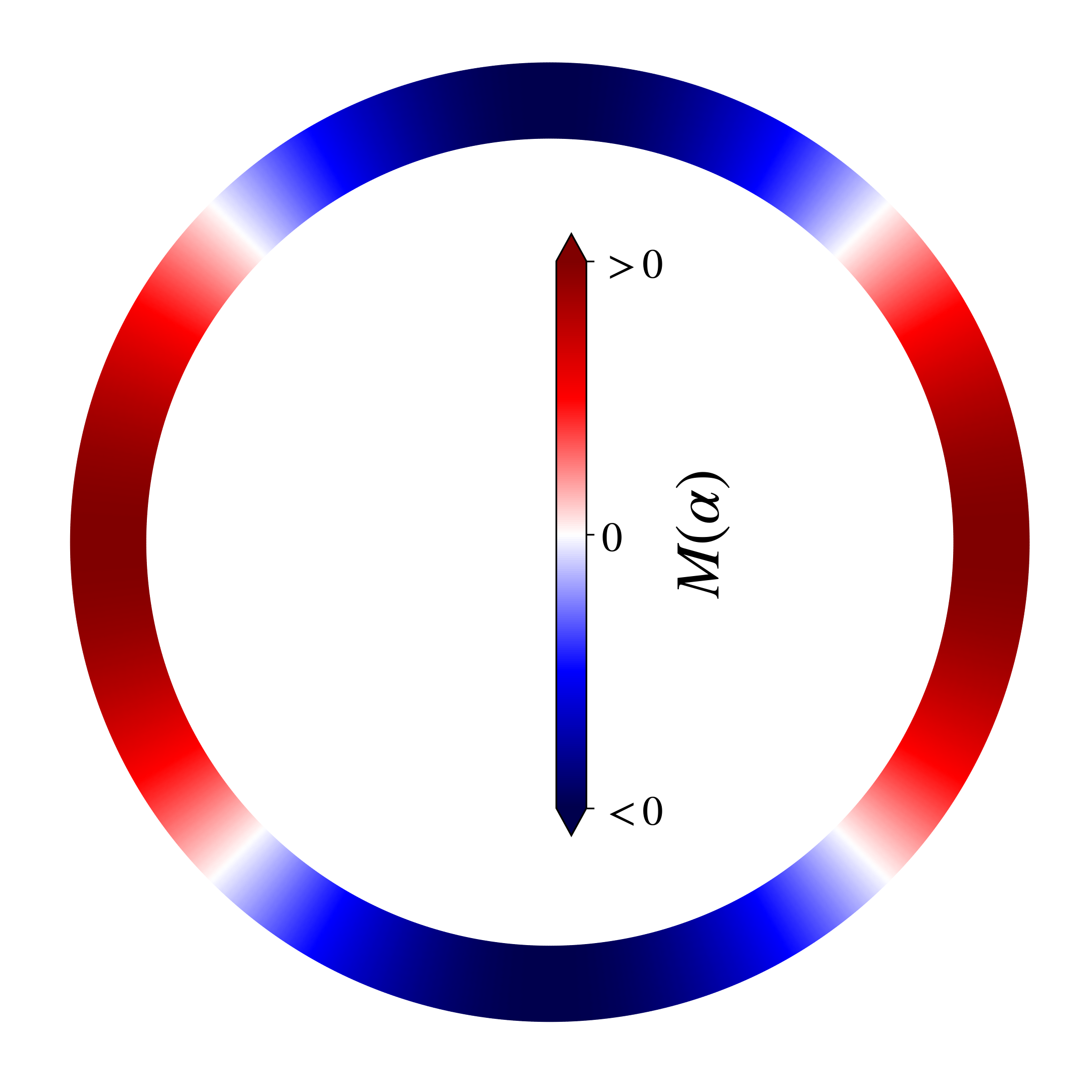
变色圆环
有时候想画一个随着角度变化的密度图,这里就给出一个例子,主要就是将matplotlib官网中的例子进行了修改
import matplotlib.tri as tri
import numpy as np
import matplotlib.pyplot as plt
from matplotlib import rcParams
import os
config = {
"font.size": 30,
"mathtext.fontset":'stix',
"font.serif": ['SimSun'],
}
rcParams.update(config) # Latex 字体设置
#---------------------------------------
def pltring():
    n_angles = 100
    n_radii = 8
    min_radius = 0.7
    radii = np.linspace(min_radius, 0.95, n_radii)

    angles = np.linspace(0, 2 * np.pi, n_angles, endpoint=False)
    angles = np.repeat(angles[..., np.newaxis], n_radii, axis=1)
    angles[:, 1::2] += np.pi / n_angles

    x = (radii * np.cos(angles)).flatten()
    y = (radii * np.sin(angles)).flatten()
    z = (np.abs(np.sin(3 * angles))).flatten()

    # Create the Triangulation; no triangles so Delaunay triangulation created.
    triang = tri.Triangulation(x, y)

    # Mask off unwanted triangles.
    triang.set_mask(np.hypot(x[triang.triangles].mean(axis=1),
                         y[triang.triangles].mean(axis=1))
                < min_radius)
    # plt.figure(figsize=(12,12))
    fig2, ax2 = plt.subplots(figsize=(10,10))
    ax2.set_aspect('equal')
    tpc = ax2.tripcolor(triang, z, shading='gouraud',cmap = "cividis_r")
    cb = fig2.colorbar(tpc,fraction = 0.045)
    cb.ax.tick_params(labelsize=20)
    plt.yticks([-1,0,1],fontproperties='Times New Roman', size = 40)
    plt.xticks([-1,0,1],fontproperties='Times New Roman', size = 40)
    # plt.show()
    picname = "phase-3.png"
    plt.savefig(picname, dpi=100, bbox_inches = 'tight')
    plt.close()
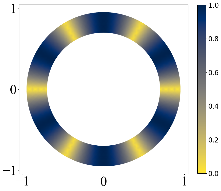
def pltring(cont):
    n_angles = 1000
    n_radii = 19
    min_radius = 0.8
    radii = np.linspace(min_radius, 0.95, n_radii)

    angles = np.linspace(0, 2 * np.pi, n_angles, endpoint=False)
    angles = np.repeat(angles[..., np.newaxis], n_radii, axis=1)
    angles[:, 1::2] += np.pi / n_angles

    x = (radii * np.cos(angles)).flatten()
    y = (radii * np.sin(angles)).flatten()
    # z = (np.abs(np.sin(3 * angles))).flatten()
    # z = ((np.cos(angles) +(-1)**cont * np.sin(angles)) * np.cos(2*angles)).flatten()
    z = (np.cos(2*angles)).flatten()

    # Create the Triangulation; no triangles so Delaunay triangulation created.
    triang = tri.Triangulation(x, y)

    # Mask off unwanted triangles.
    triang.set_mask(np.hypot(x[triang.triangles].mean(axis=1),
                         y[triang.triangles].mean(axis=1))
                < min_radius)
    # plt.figure(figsize=(12,12))
    fig2, ax2 = plt.subplots(figsize=(10,10))
    ax2.set_aspect('equal')
    tpc = ax2.tripcolor(triang, z, shading='gouraud',cmap = "seismic")
    cb = fig2.colorbar(tpc,fraction = 0.045,ticks=[-1, 0, 1],extend='both',label = r"$M(\alpha)$")
    cb.ax.tick_params(labelsize = 20)
    cb.ax.set_yticklabels([r'$<0$', r'$0$', r'$>0$'])
    cb.ax.set_position([0.48, 0.3, 0.3, 0.4])
    plt.yticks([],fontproperties='Times New Roman', size = 40)
    plt.xticks([],fontproperties='Times New Roman', size = 40)
    # plt.show()
    ax = plt.gca()
    ax.spines["bottom"].set_linewidth(0)
    ax.spines["left"].set_linewidth(0)
    ax.spines["right"].set_linewidth(0)
    ax.spines["top"].set_linewidth(0)

    picname = "mass-" + str(cont) + ".png"
    plt.savefig(picname, dpi = 300, bbox_inches = 'tight',transparent = True)
    plt.close()
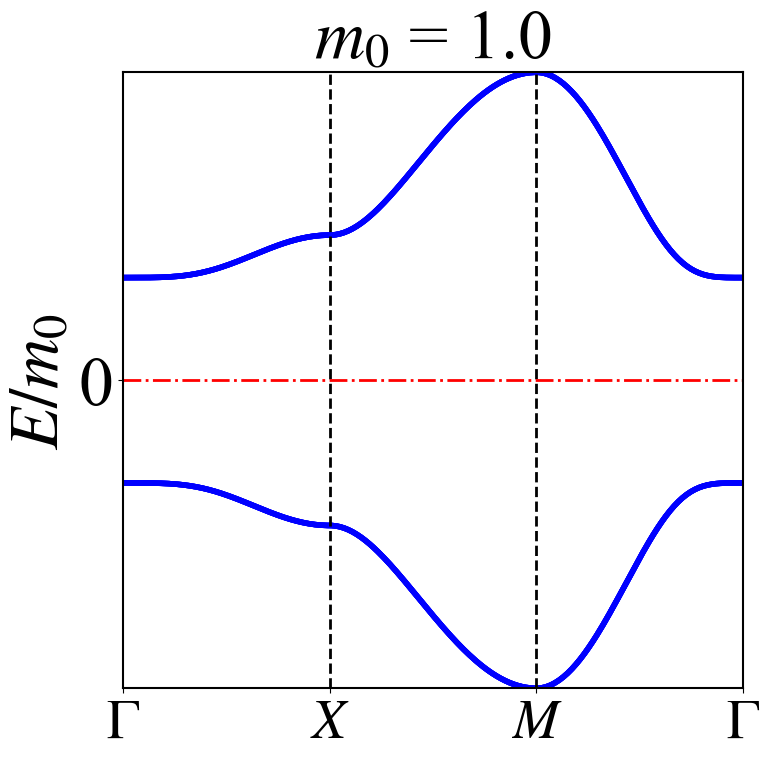
高对称路径能带图
import numpy as np
import matplotlib.pyplot as plt
from matplotlib import rcParams
import os
config = {
"font.size": 40,
"mathtext.fontset":'stix',
"font.serif": ['SimSun'],
}
rcParams.update(config) # Latex 字体设置
#------------------------------------
def Pauli():
    s0 = np.array([[1,0],[0,1]])
    sx = np.array([[0,1],[1,0]])
    sy = np.array([[0,-1j],[1j,0]])
    sz = np.array([[1,0],[0,-1]])
    return s0,sx,sy,sz
#-----------------------------------
def hamset(kx,ky,m0):
    hn = 8
    s0 = np.zeros([2,2],dtype = complex)
    sx = np.zeros([2,2],dtype = complex)
    sy = np.zeros([2,2],dtype = complex)
    sz = np.zeros([2,2],dtype = complex)
    ham = np.zeros([hn,hn],dtype = complex)
    # m0 = 1.5
    tx = 1.0
    ty = 1.0
    ax = 1.0
    ay = 1.0
    d0 = 0.0
    dx = 0.5
    dy = -dx
    s0,sx,sy,sz = Pauli()
    ham = (m0 - tx*np.cos(kx) - ty*np.cos(ky))*np.kron(np.kron(s0,sz),sz) + ax*np.sin(kx)*np.kron(np.kron(sz,sx),s0)\
            + ay*np.sin(ky)*np.kron(np.kron(s0,sy),sz) + (d0 + dx*np.cos(kx) + dy*np.cos(ky))*np.kron(np.kron(sy,s0),sy)
    return ham
#------------------------------------------------------------------------------------
def engvals(kx,ky,m0):
    # 求解本征值,python给出的是个复数,还不按照顺序排列,很烦
    ham  = hamset(kx,ky,m0)
    vals = np.linalg.eigvals(ham)
    # print(vals.real)
    return sorted(vals.real)
#----------------------------------------------------------------------------------------------------
def HSP2(m0):
    kxlist = np.linspace(0,np.pi,100)
    relist1 = []
    x0 = []
    for kx in kxlist:
        x0.append(kx/np.pi)
        vals = engvals(kx,0,m0)
        relist1.append(vals)
    for ky in kxlist:
        x0.append(ky/np.pi + 1)
        vals = engvals(np.pi,ky,m0)
        relist1.append(vals)
    for k in kxlist:
        x0.append(k/np.pi + 2)
        vals = engvals(np.pi - k,np.pi - k,m0)
        relist1.append(vals)

    plt.figure(figsize=(8,8))
    # plt.plot(x0,y01,c = "blue" ,lw = 4,label = r"$\tilde{M}^+_I\times \tilde{M}^+_{II}$")
    # plt.plot(x0,y02,c = "red" ,lw = 4,label = r"$\tilde{M}^-_I\times \tilde{M}^-_{II}$")
    plt.plot(x0,relist1,c = "blue" ,lw = 4)
    # plt.plot(x0,y02,c = "red" ,lw = 4,label = r"$\tilde{M}^-$")
    font2 = {'family': 'Times New Roman',
             'weight': 'normal',
             'size': 50,
             }
    x0min = np.min(x0)
    x0max = np.max(x0)
    y0max = np.max(relist1)
    # plt.ylim(yaxmin,yaxman + 0.25)
    # plt.text(pp1 - 0.2,-0.8,r"$0.23\pi$",color = "green")
    # plt.text(pp2 ,-0.8,r"$0.27\pi$",color = "green")
    plt.vlines(2,ymin = -y0max,ymax = y0max,lw = 2,colors = "black",ls = "--")
    plt.vlines(1,ymin = -y0max,ymax = y0max,lw = 2,colors = "black",ls = "--")
    plt.hlines(0,xmin = x0min,xmax = x0max,lw = 2,colors = "red",ls = "-.")
    xtic = [0,1,2,3]
    xticlab = ["$\Gamma$",r"$X$","$M$","$\Gamma$"]
    plt.xticks(xtic,list(xticlab),fontproperties='Times New Roman', size = 40)
    plt.yticks([-5,0,5],fontproperties='Times New Roman', size = 50)
    plt.ylabel("$E/m_0$", font2)
    plt.xlim(x0min,x0max)
    plt.ylim(-y0max,y0max)
    tit = "$m_0$ = " + str(m0)
    plt.title(tit,font2)
    # plt.legend(loc = 'upper right', ncol = 1, shadow = True, fancybox = True, prop = font1, markerscale = 0.5) # 图例
    # ax1.patch.set_facecolor("lightblue")    # 设置 ax1 区域背景颜⾊
    # ax1.patch.set_alpha(0.5)    # 设置 ax1 区域背景颜⾊透明度
    # plt.show()
    ax = plt.gca()
    # ax.patch.set_facecolor("lightblue")    # 设置 ax1 区域背景颜⾊
    # ax.patch.set_alpha(0.5)    # 设置 ax1 区域背景颜⾊透明度
    ax.spines["bottom"].set_linewidth(1.5)
    ax.spines["left"].set_linewidth(1.5)
    ax.spines["right"].set_linewidth(1.5)
    ax.spines["top"].set_linewidth(1.5)
    picname = "hsp2-" + str(format(m0,".2f")) + ".png"
    plt.savefig(picname, dpi = 100, bbox_inches = 'tight')
    plt.close()

#----------------------------------------------------------------
if __name__=="__main__":
    HSP2(1.)
    # engvals(0.1,0.1,1)
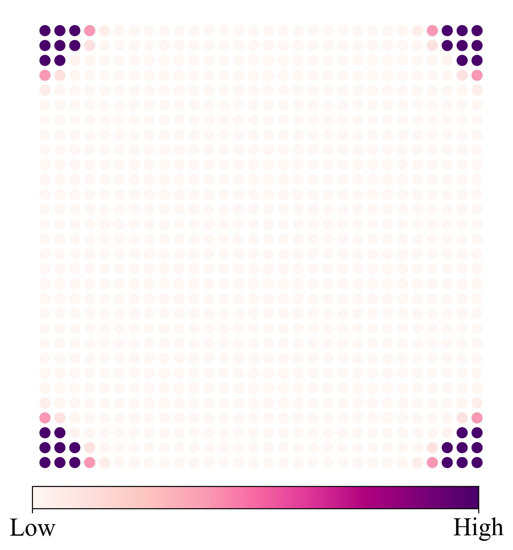
密度图2
def ldosplt(cont):
    dataname = "wave-30.00-Jx-" + str(cont) + ".dat"
    # picname = "ldos-" + str(cont) + ".png"
    picname = os.path.splitext(dataname)[0] + "-2" + ".png"
    os.chdir(os.getcwd())# 确定用户执行路径
    x0 = []
    y0 = []
    z0 = []
    z1 = []
    with open(dataname) as file:
        da = file.readlines()
        for f1 in da:
            if len(f1) > 3:
                ldos = [float(x) for x in f1.strip().split()]
                x0.append(ldos[0])
                y0.append(ldos[1])
                z0.append(ldos[4] + ldos[5] + ldos[6] + ldos[7])
    z0min = np.max(z0)
    z0max = np.max(z0)
    z0 = (z0 - np.min(z0))/(np.max(z0) - np.min(z0))*400 # 数据归一化
    plt.figure(figsize=(8, 9))
    # sc = plt.scatter(x0, y0, c = z0,s = z0,vmin = 0, vmax = z0max,cmap = "bwr",edgecolor = "black")
    sc = plt.scatter(x0, y0, c = z0,s = 60,vmin = 0, vmax = z0max,cmap = "RdPu")
    # sc = plt.scatter(x0, y0, c = z0,s = z0,vmin  = 0, vmax = z0max,cmap="BuPu")
    cb = plt.colorbar(sc,fraction = 0.1,ticks=[ 0, z0max],orientation='horizontal')  # 调整colorbar的大小和图之间的间距
    cb.ax.set_xticklabels(['Low', 'High'])
    cb.ax.set_position([0.2, 0.2, 0.61, 0.1])
    cb.ax.tick_params(labelsize=20)
    font2 = {'family': 'Times New Roman',
             'weight': 'normal',
             'size': 40,
             }
    # cb.set_label('ldos',fontdict=font2) #设置colorbar的标签字体及其大小
    # plt.scatter(x0, y0, s = 5, color='blue',edgecolor="blue")
    plt.axis('scaled')
    # plt.xlabel("x",font2)
    # plt.ylabel("y",font2)
    # tit = "$h_x= " + str(cont) + "$"
    # plt.title(tit,font2)
    plt.yticks([],fontproperties='Times New Roman', size = 40)
    plt.xticks([],fontproperties='Times New Roman', size = 40)
    plt.tick_params(axis='x',width = 0,length = 10)
    plt.tick_params(axis='y',width = 0,length = 10)
    ax = plt.gca()
    ax.spines["bottom"].set_linewidth(0)
    ax.spines["left"].set_linewidth(0)
    ax.spines["right"].set_linewidth(0)
    ax.spines["top"].set_linewidth(0)
    plt.savefig(picname, dpi = 300,bbox_inches = 'tight')
    plt.close()
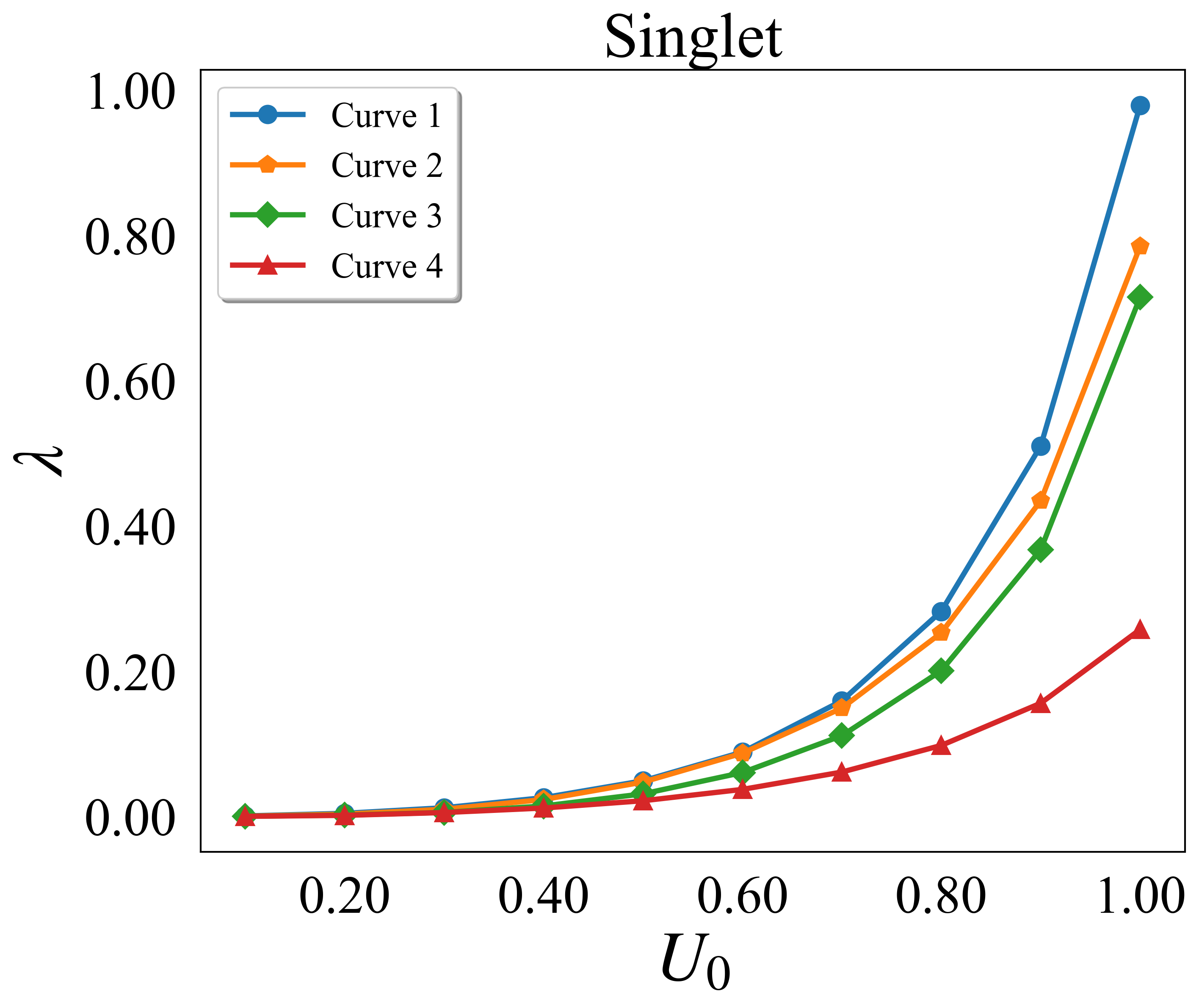
线图+scatter
import numpy as np
import matplotlib.pyplot as plt
from matplotlib import rcParams
import matplotlib.cm as cm
import os
import matplotlib.ticker as mticker
#----------------------------------------------------------
def lambda_singlet():
    dataname = "singlet.dat"
    picname = os.path.splitext(dataname)[0] + ".png"
    da = np.loadtxt(dataname)
    x0 = np.linspace(0.1,1,10)
    plt.figure(figsize = (10,8))
    plt.title("Singlet")

    # labels = [r"$p_x$",r"$p_y$",r"$f_x$",r"$f_y$"]
    labels = []
    for i in range(len(da[1, :])):
        labels.append(f"Curve {i+1}")  # Create informative labels

    for i0 in range(len(da[1, :])):
        marker_style = ['o', 'p', 'D', '^', 's'][i0 % len(['o', 'p', 'D', '^', 's'])]
        plt.plot(x0, da[:, i0], marker = marker_style, label = labels[i0],lw = 3, markersize = 10)  # Use labels in plot and legend


    # plt.plot(x0,da)
    # marker_styles = ['o', 'p', 'D', '^', 's']
    # for i0 in range(len(da[1,:])):
    #     marker_style = marker_styles[i0 % len(marker_styles)]
    #     # plt.scatter(x0,da[:,i0],s = 100,marker = marker_style)
    #     plt.scatter(x0,da[:,i0],s = 100)

    font1 = {'family': 'Times New Roman','weight': 'normal','size': 20}
    font2 = {'family': 'Times New Roman','weight': 'normal','size': 40}
    plt.ylabel(r"$\lambda$",font2) # 调整标签到坐标轴距离
    plt.xlabel(r"$U_0$",font2)

    # Set X-Axis Precision
    x_formatter = mticker.FormatStrFormatter(f"%.{2}f")  # Set precision to 2 decimal places
    x_locator = mticker.MaxNLocator(nbins=5)  # Set number of ticks to 5


    # Set Y-Axis Precision
    y_formatter = mticker.FormatStrFormatter(f"%.{2}f")  # Set precision to 3 significant digits
    y_locator = mticker.AutoLocator()  # Use automatic tick placement

    plt.legend(loc='upper left', shadow=True, fancybox=True,prop = font1)
    plt.tick_params(axis='x',width = 0,length = 10)
    plt.tick_params(axis='y',width = 0,length = 10)
    ax = plt.gca()
    ax.xaxis.set_major_formatter(x_formatter)
    ax.xaxis.set_major_locator(x_locator)
    ax.yaxis.set_major_formatter(y_formatter)
    ax.yaxis.set_major_locator(y_locator)
    ax.spines["bottom"].set_linewidth(1)
    ax.spines["left"].set_linewidth(1)
    ax.spines["right"].set_linewidth(1)
    ax.spines["top"].set_linewidth(1)
    plt.savefig(picname, dpi = 300,bbox_inches = 'tight',transparent = True)
    # plt.show()
    plt.close()
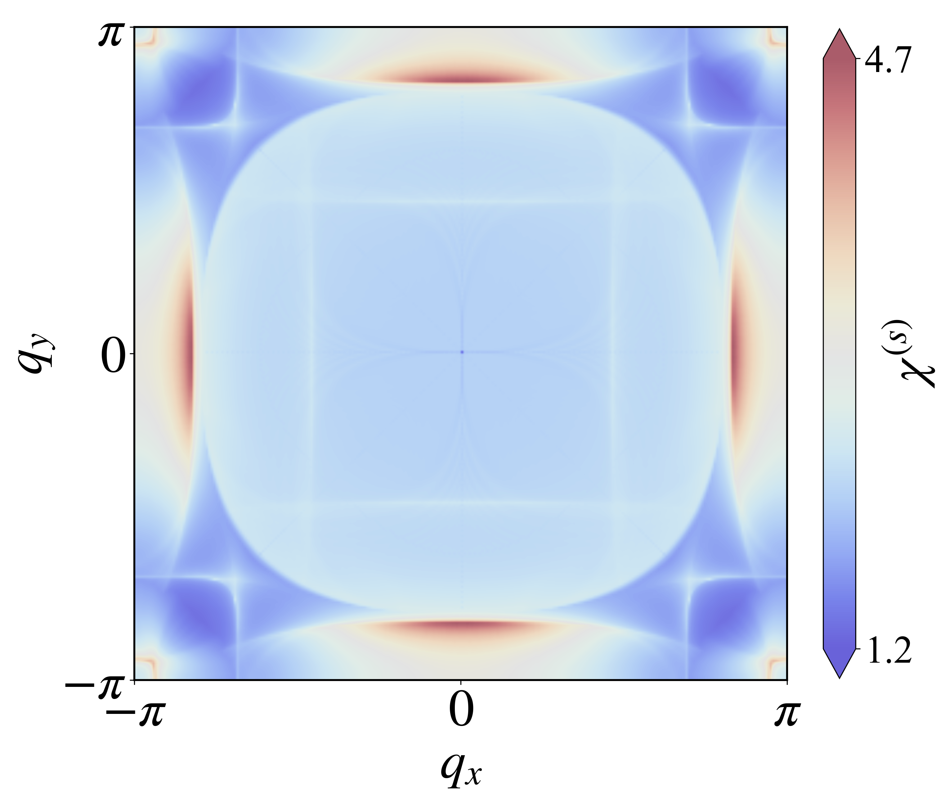
自定义colorbar
def plotchi2(numk):
    dataname = "chi-val-kn-" + str(format(numk,"0>3d")) + ".dat"
    picname = os.path.splitext(dataname)[0] + ".png"
    da = np.loadtxt(dataname)
    x0 = da[:,0]
    z0 = np.array(da[:,2])
    xn = int(np.sqrt(len(x0)))
    z0 = z0.reshape(xn,xn)
    plt.figure(figsize = (10,10))

    # Create custom colormap from Rainbow colormap
    # Define colors
    light = 0.7    #  控制颜色亮度    RGBA-->A   alpha
    colors1 = np.array([[0.163302, 0.12, 0.79,light], [0.25, 0.31, 0.89,light], [0.41, 0.54, 0.94,light],
                    [0.57, 0.73, 0.95,light], [0.72, 0.86, 0.93,light], [0.83, 0.90, 0.87,light],[0.85,0.85,0.85,light],
                    [0.89, 0.88, 0.77,light], [0.91, 0.79, 0.65,light], [0.87, 0.64, 0.52,light],
                    [0.80, 0.45, 0.39,light], [0.69, 0.24, 0.27,light], [0.53, 0.09, 0.17,light]])
    cmap = colors.LinearSegmentedColormap.from_list('', colors1)

    sc = plt.imshow(z0,interpolation='bilinear', cmap = cmap,origin='lower', extent=[-np.pi, np.pi, -np.pi, np.pi],vmax = z0.max(), vmin = z0.min())
    # sc = plt.imshow(z0,interpolation='bilinear', cmap = "jet",origin='lower')
    cb = plt.colorbar(sc,fraction = 0.045,extend = 'both',ticks = [np.min(z0),np.max(z0)])  # 调整colorbar的大小和图之间的间距
    cb.ax.set_yticklabels([format(np.min(z0),".1f"),format(np.max(z0),".1f")])
    cb.ax.tick_params(labelsize = 30)   # 消除colorbar上的刻度
    cb.set_label(r"$\chi^{(s)}$", labelpad = -25,loc = "center",size = 40)
    # cb.ax.set_position([0.77, 0.2, 0.8, 0.6])
    font2 = {'family': 'Times New Roman','weight': 'normal','size': 40}
    plt.axis('scaled')
    plt.xlabel(r"$q_x$",font2)
    plt.ylabel(r"$q_y$",font2)
    # tit = "$J_x= " + str(cont) + "$"
    # plt.title(tit,font2)
    xtic = [-np.pi,0,np.pi]
    xticlab = ["$-\pi$","$0$","$\pi$"]
    plt.xticks(xtic,list(xticlab),fontproperties='Times New Roman', size = 40)
    plt.yticks(xtic,list(xticlab),fontproperties='Times New Roman', size = 40)
    # plt.tick_params(axis='x',width = 2,length = 10)
    # plt.tick_params(axis='y',width = 2,length = 10)
    ax = plt.gca()
    ax.spines["bottom"].set_linewidth(1.5)
    ax.spines["left"].set_linewidth(1.5)
    ax.spines["right"].set_linewidth(1.5)
    ax.spines["top"].set_linewidth(1.5)
    # plt.show()
    plt.savefig(picname, dpi = 300,bbox_inches = 'tight')
    plt.close()
公众号
相关内容均会在公众号进行同步,若对该Blog感兴趣,欢迎关注微信公众号。
