做数值计算好用的软件及杂项整理
软件下载
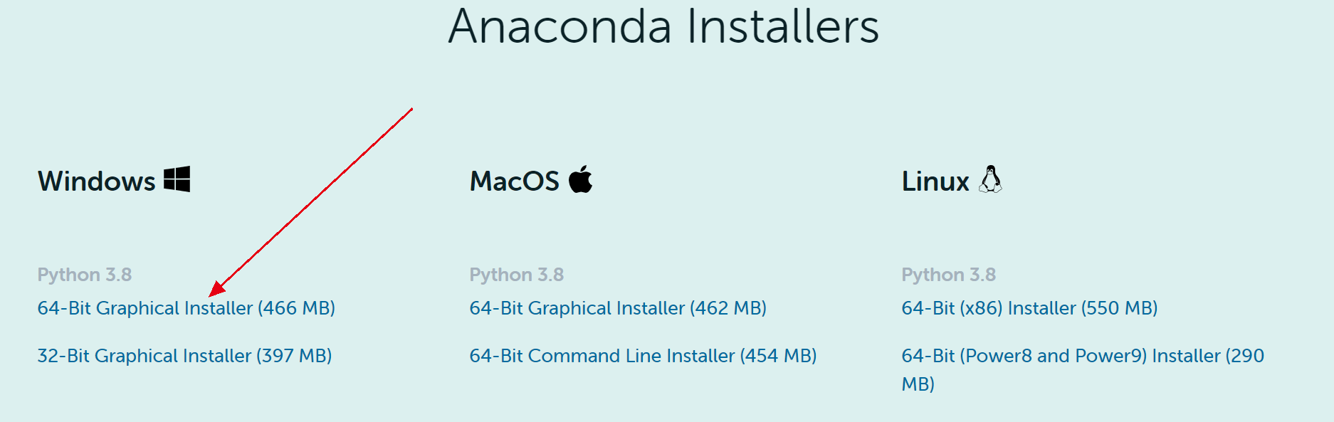
安装过程
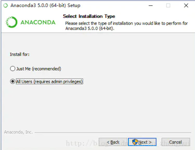
1)在“Select Installation Type”界面的“Install for”中选择“All Users(requires admin privileges)”单选按钮
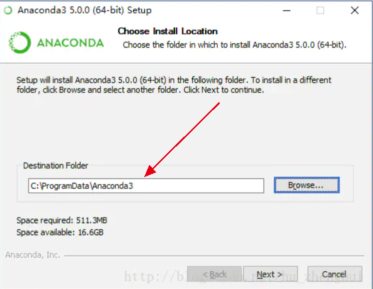
2)在“Choose Install Location”界面中查看“Destination Folder”,可能为C:\ProgramData\Anaconda3,注意检查该路径不能包含非英文字符
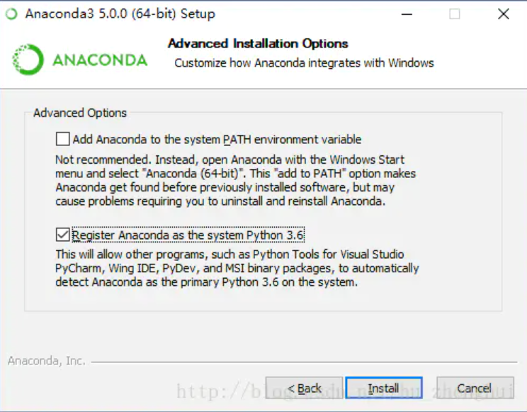
3)在“Advanced Installation Options”界面中选中“Register Anaconda as my default Python 3.6”复选框。
!png
建议这里不要选则将Anaconda增加到系统的环境变量中,增加太多会导致系统上的环境变量较为混乱.如果单独出来,后面对于Anaconda的包管理来说,也是较为简洁的,可以通过它自带的命令行来进行包管理.
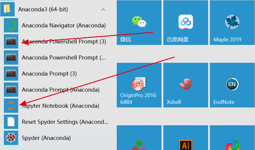
4)安装完成后,开始==>所有程序中,出现文件夹anaconda3(64-bit)
Anaconda包管理
1.包更新升级
1
conda upgrade --all
2.包安装
1
2
3
conda install numpy scipy pandas
conda install numpy=1.10 安装指定版本的包3.包移除
1
conda remove package_name
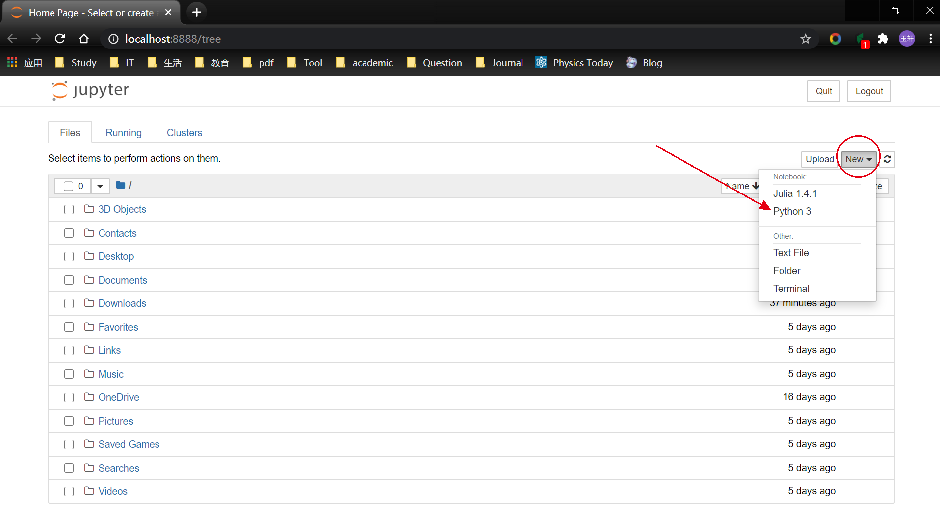
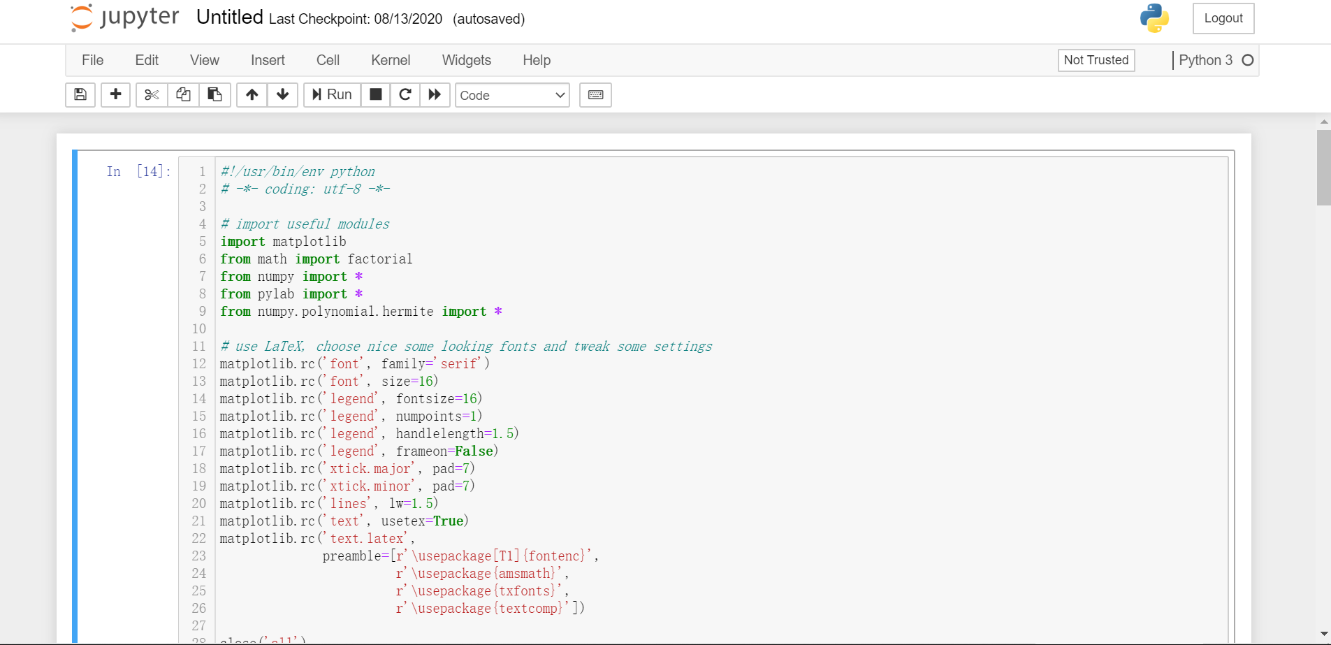
Jupyter使用
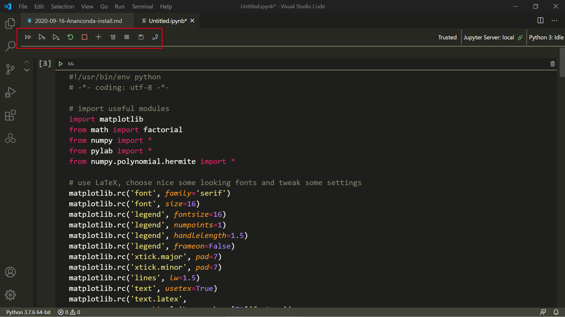
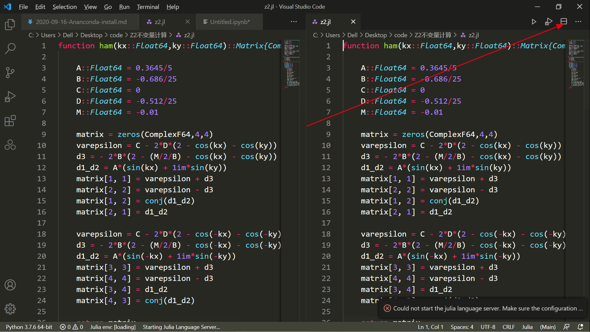
VsCode使用
Plotly
Installation
1 | pip install plotly==4.10.0 |
Jupyter Notebook Support
1 | conda install "notebook>=5.3" "ipywidgets>=7.2" |
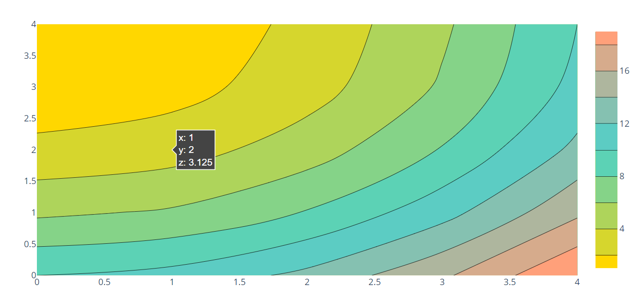
plot
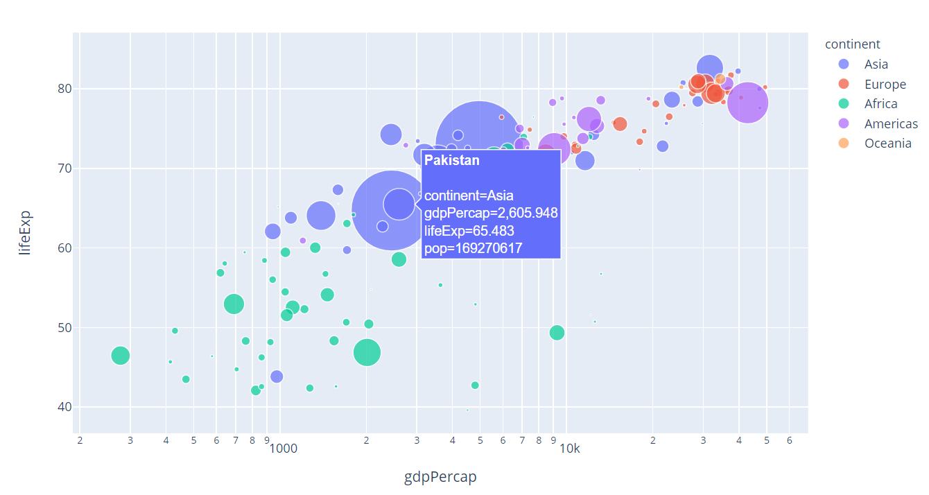
1 | import plotly.graph_objects as go |
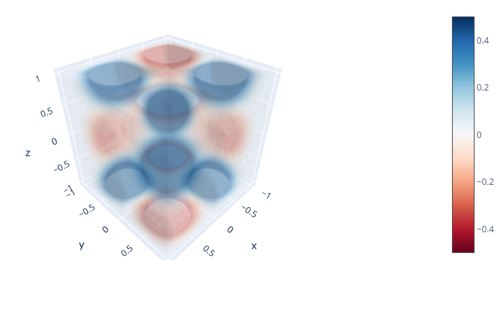
体积图
1 | import plotly.graph_objects as go |
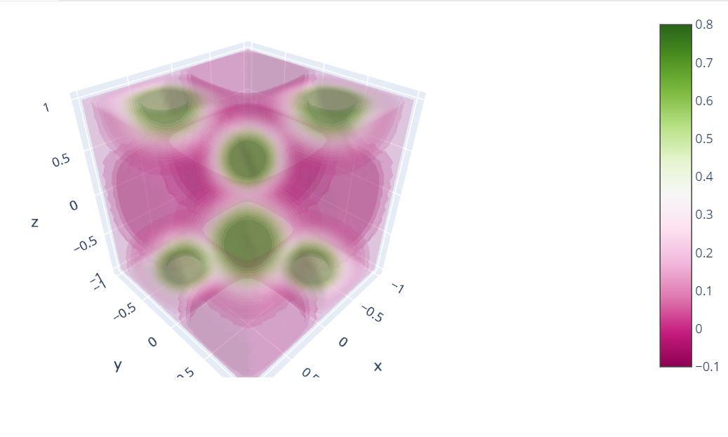
1 | import plotly.graph_objects as go |
服务器程序编译执行
Linux基本命令
1 | ls or ls -al 显示当前文件夹中的所有文件 |
新手可以先在本地将程序写好之后传到服务器端进行编译运行,或者使用Xshell之后可以直接使用gedit在服务器端利用图形界面对代码进行直接修改,vim使用需要一定的学习.
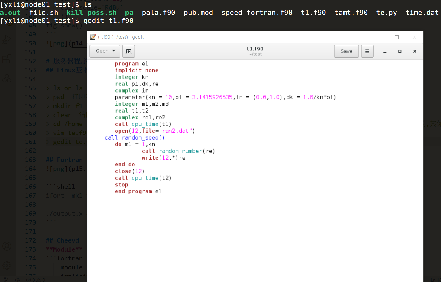
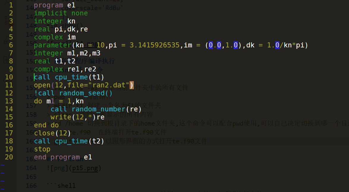
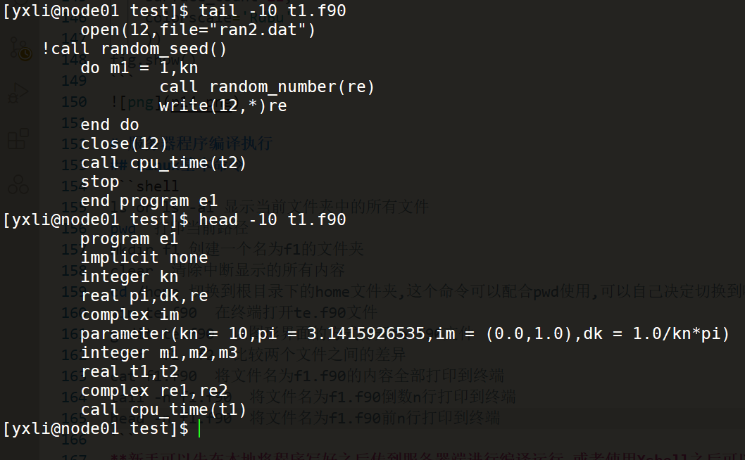
Fortran
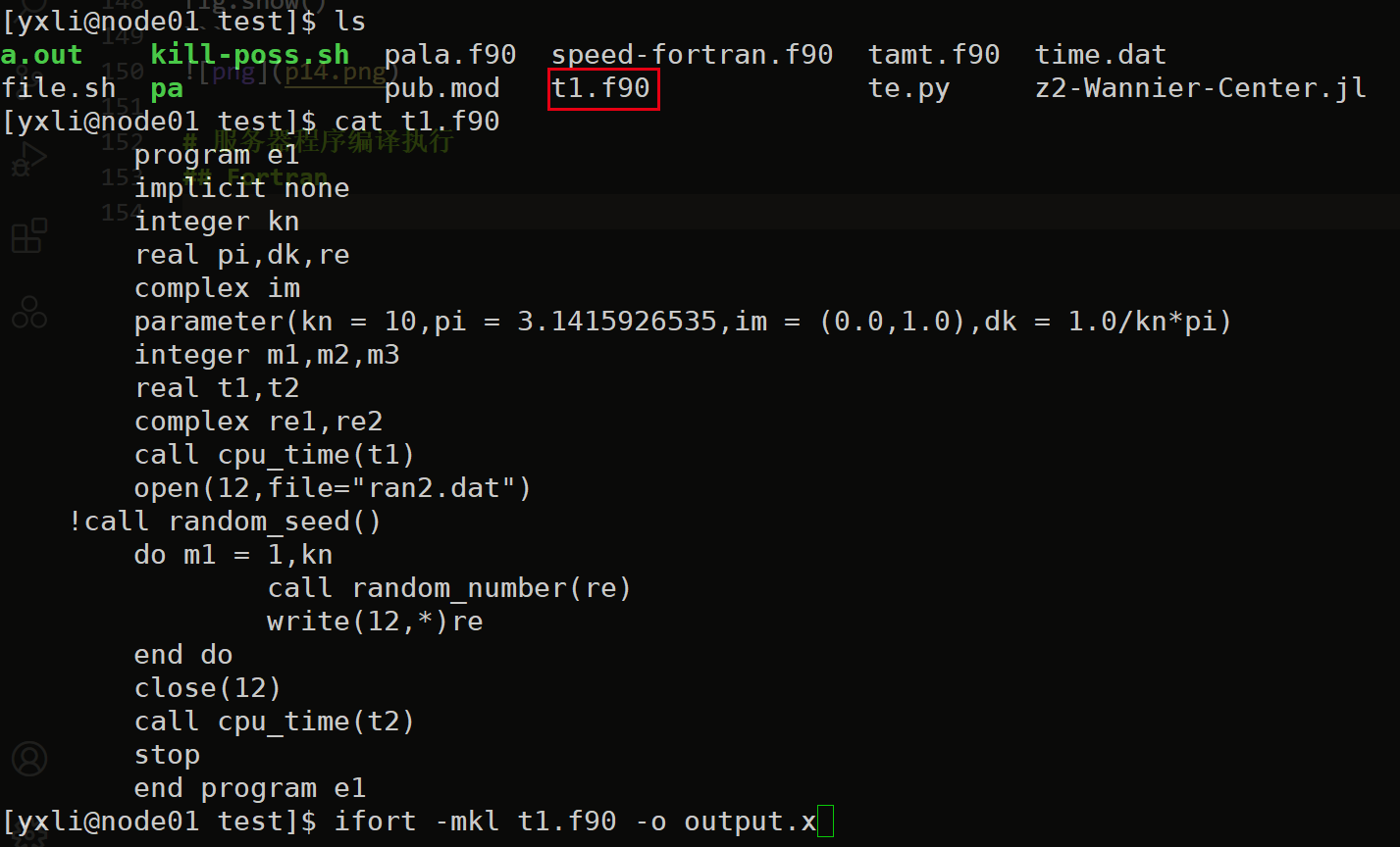
1 | ifort -mkl t1.f90 -o output.x 编译t1.f90文件,生成可执行文件output.x |
Cheevd
Module1
2
3
4
5
6
7
8
9
10
11
12
13
14
15
16module pub
implicit none
integer xn,yn,ne
parameter(xn = 30,yn = 30,ne = 1000)
integer,parameter::N = xn*yn*8
integer::lda = N
integer,parameter::lwmax=2*N+N**2
real,allocatable::w(:)
complex*8,allocatable::work(:)
real,allocatable::rwork(:)
integer,allocatable::iwork(:)
integer lwork ! at least 2*N+N**2
integer lrwork ! at least 1 + 5*N +2*N**2
integer liwork ! at least 3 +5*N
integer info
end module pub
对角化函数调用1
2
3
4
5
6
7
8
9
10
11
12
13
14
15
16
17
18
19
20
21
22
23subroutine eigsol()
use pub
integer m
lwork = -1
liwork = -1
lrwork = -1
call cheevd('V','Upper',N,Ham,lda,w,work,lwork,rwork,lrwork,iwork,liwork,info)
lwork = min(2*N+N**2, int( work( 1 ) ) )
lrwork = min(1+5*N+2*N**2, int( rwork( 1 ) ) )
liwork = min(3+5*N, iwork( 1 ) )
call cheevd('V','Upper',N,Ham,lda,w,work,lwork,rwork,lrwork,iwork,liwork,info)
if( info .GT. 0 ) then
open(11,file="mes.txt",status="unknown")
write(11,*)'The algorithm failed to compute eigenvalues.'
close(11)
end if
open(12,file="eigval.dat",status="unknown")
do m = 1,N
write(12,*)m,w(m)
end do
close(12)
return
end subroutine eigsol
程序示例1
2
3
4
5
6
7
8
9
10
11
12
13
14
15
16
17
18
19
20
21
22
23
24
25
26
27
28
29
30
31
32
33
34
35
36
37
38
39
40
41
42
43
44
45
46
47
48
49
50
51
52
53
54
55
56
57
58
59
60
61
62
63
64
65
66
67
68
69
70
71
72
73
74
75
76
77
78
79
80
81
82
83
84
85
86
87
88
89
90
91
92
93
94
95
96
97
98
99
100
101
102
103
104
105
106
107
108
109
110
111
112
113
114
115
116
117
118
119
120
121
122
123
124
125
126
127
128
129
130
131
132
133
134
135
136
137
138
139
140
141
142
143
144
145
146
147! Author:YuXuanLi
! E-Mail:yxli406@gmail.com
! Article:Majorana Corner Modes in a High-Temperature Platform
! Doi:10.1103/PhysRevLett.121.096803
!==========================================
module param
implicit none
integer xn,yn,nkx,nky,ne,nkxy
parameter(nkx=50,nky=50,ne=1000)
integer,parameter::N = 4
complex,parameter::im = (0.,1.) !Imagine unit
real,parameter::pi = 3.14159265358979
complex Ham(N,N) ! Hamiltonian Matrix
real mu ! Chemical Potential
real tx,ty ! hopping term energy
real ax,ay ! copule energy
real m0 !Driac mass
real kx,ky
! LAPACK PACKAGE PARAM
integer::lda = N
integer,parameter::lwmax = 2*N+N**2
real,allocatable::w(:)
complex,allocatable::work(:)
real,allocatable::rwork(:)
integer,allocatable::iwork(:)
integer lwork ! at least 2*N+N**2
integer lrwork ! at least 1 + 5*N +2*N**2
integer liwork ! at least 3 +5*N
integer info
end module param
!========== PROGRAM START ==========================
program sol
use param
integer m,l ! loop variales
!================ Physics memory allocate =================
allocate(w(N))
allocate(work(lwmax))
allocate(rwork(1+5*N+2*N**2))
allocate(iwork(3+5*N))
! paramater set value
m0 = 1.5 ! effective mass
tx = 1.0 ! hopping energy in x direction
ty = 1.0 ! hopping energy in y direction
mu = 0.2 ! chemical potential
ax = 1.0 ! couple energy in x direction
ay = 1.0 ! couple energy in y direction
call band()
stop
end program
!===========================================================
subroutine matrix_set()
use param
Ham = 0
!----------------------------------------------
Ham(1,1) = m0 - tx*cos(kx) - ty*cos(ky) + mu
Ham(2,2) = -(m0 - tx*cos(kx) - ty*cos(ky)) + mu
Ham(3,3) = m0 - tx*cos(kx) - ty*cos(ky) + mu
Ham(4,4) = -(m0 - tx*cos(kx) - ty*cos(ky)) + mu
!-----------------------------------------------
Ham(1,2) = ax*sin(kx) - im*ay*sin(ky)
Ham(2,1) = ax*sin(kx) + im*ay*sin(ky)
Ham(3,4) = -ax*sin(kx) - im*ay*sin(ky)
Ham(4,3) = -ax*sin(kx) + im*ay*sin(ky)
!--------------------------------------------------
call ishermitian()
end subroutine matrix_set
!============================================================
subroutine band()
! Evaluate the density of state in (x,y) position
use param
integer m,l,k,i! circle variable
open(12,file="tiband.dat")
! (0,0)------>(pi,0)
do k = 0,nky
kx = pi*k/nkx ! discrete wavevector in x direction
!kx = 0
ky = 0 ! discrete wavevector in y direction
! 不同的kx和ky重新进行哈密顿量矩阵的构造和求解
call matrix_set() ! 新的kx和ky下重新填充矩阵,并求解对应本征值
call eigSol()
write(12,"(6f9.5)")kx,ky,(w(i),i=1,N)
end do
! (pi,0)---->(pi,pi)
do k = 0,nkx
kx = pi
ky = pi*k/nkx ! discrete wavevector in y direction
! 不同的kx和ky重新进行哈密顿量矩阵的构造和求解
call matrix_set() ! 新的kx和ky下重新填充矩阵,并求解对应本征值
call eigSol()
write(12,"(6f9.5)")kx,ky,(w(i),i=1,N)
end do
! (pi,pi)---->(0,0)
do k = 0,nkx-1
kx = pi-pi*k/nkx ! discrete wavevector in x direction
ky = pi-pi*k/nky ! discrete wavevector in y direction
call matrix_set() ! 新的kx和ky下重新填充矩阵,并求解对应本征值
call eigSol()
write(12,"(6f9.5)")kx,ky,(w(i),i=1,N)
end do
close(12)
end subroutine band
!============================================================
subroutine ishermitian()
use param
integer i,j
integer ccc
ccc = 0
open(16,file = 'verify.dat')
do i = 1,N
do j = 1,N
if (Ham(i,j) .ne. conjg(Ham(j,i)))then
ccc = ccc +1
write(16,*)i,j
write(16,*)Ham(i,j)
write(16,*)Ham(j,i)
end if
end do
end do
write(16,*)ccc
close(16)
return
end subroutine ishermitian
!================= Hermitain Matrices solve ==============
subroutine eigSol()
use param
integer m
lwork = -1
liwork = -1
lrwork = -1
call cheevd('V','Upper',N,Ham,lda,w,work,lwork,rwork,lrwork,iwork,liwork,info)
lwork = min(2*N+N**2, int( work( 1 ) ) )
lrwork = min(1+5*N+2*N**2, int( rwork( 1 ) ) )
liwork = min(3+5*N, iwork( 1 ) )
call cheevd('V','Upper',N,Ham,lda,w,work,lwork,rwork,lrwork,iwork,liwork,info)
if( info .GT. 0 ) then
open(101,file="mes.txt",status="unknown")
write(101,*)'The algorithm failed to compute eigenvalues.'
close(101)
end if
open(100,file="eigval.dat",status="unknown")
do m = 1,N
write(100,*)m,w(m)
end do
close(100)
return
end subroutine eigSol
Python
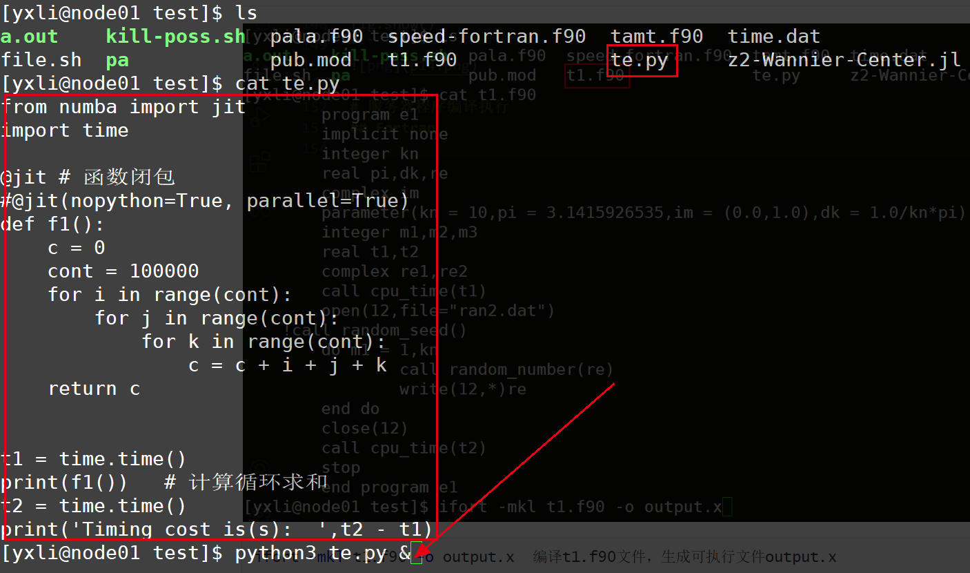
1
2
3python3 te.py & 执行python程序,并放到后台执行(python不用编译)
julia的执行和python相同
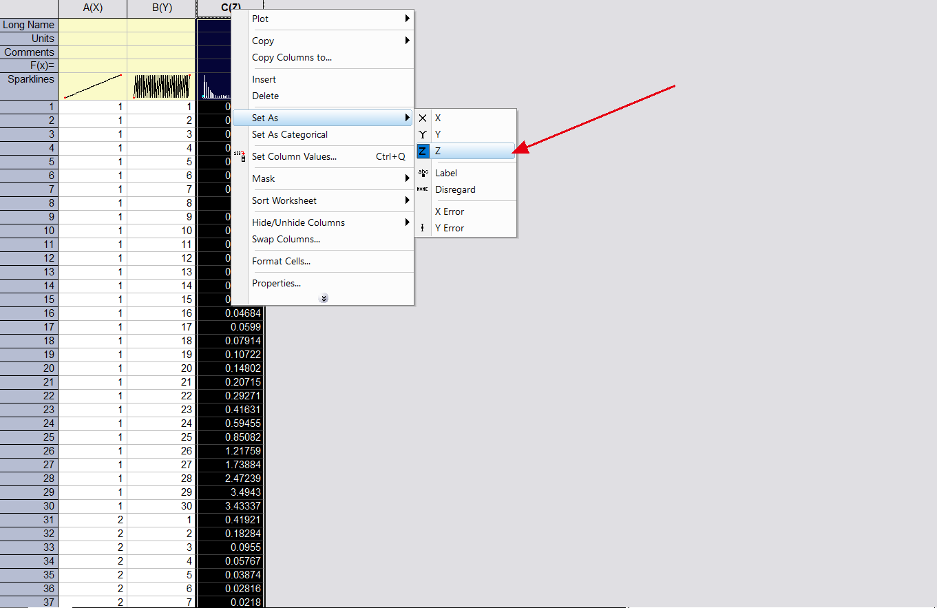
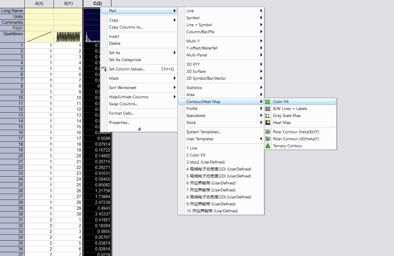
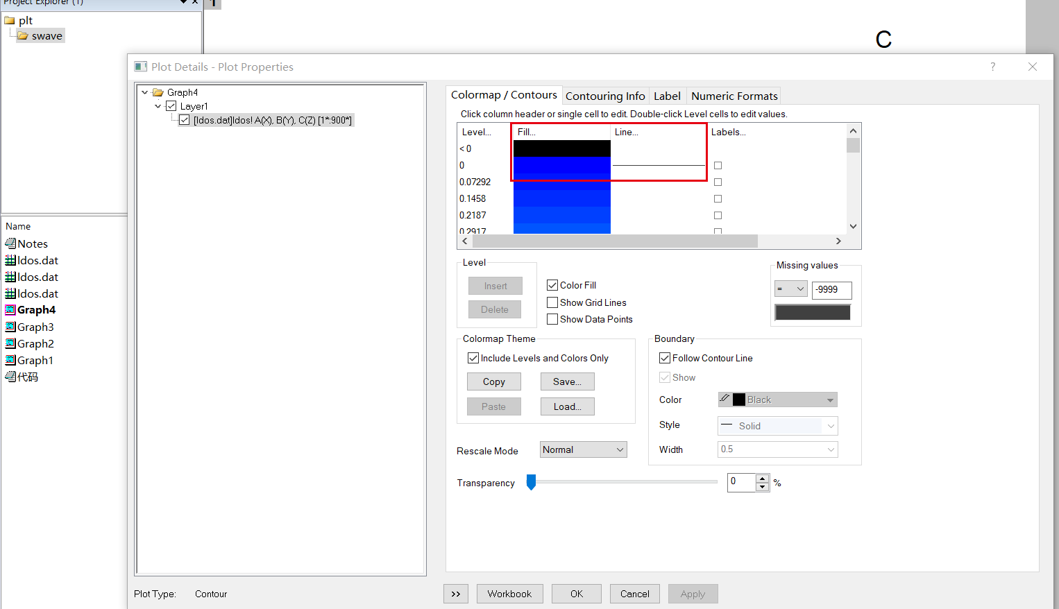
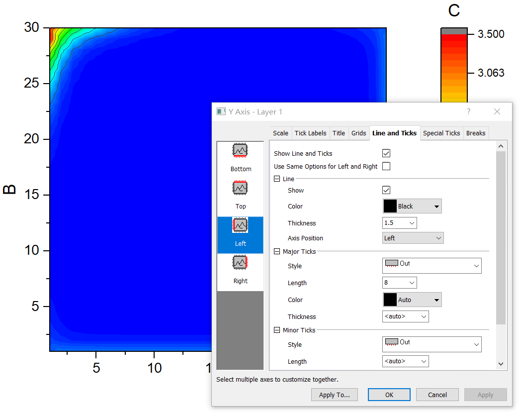
Origin作图
坐标轴样式调节
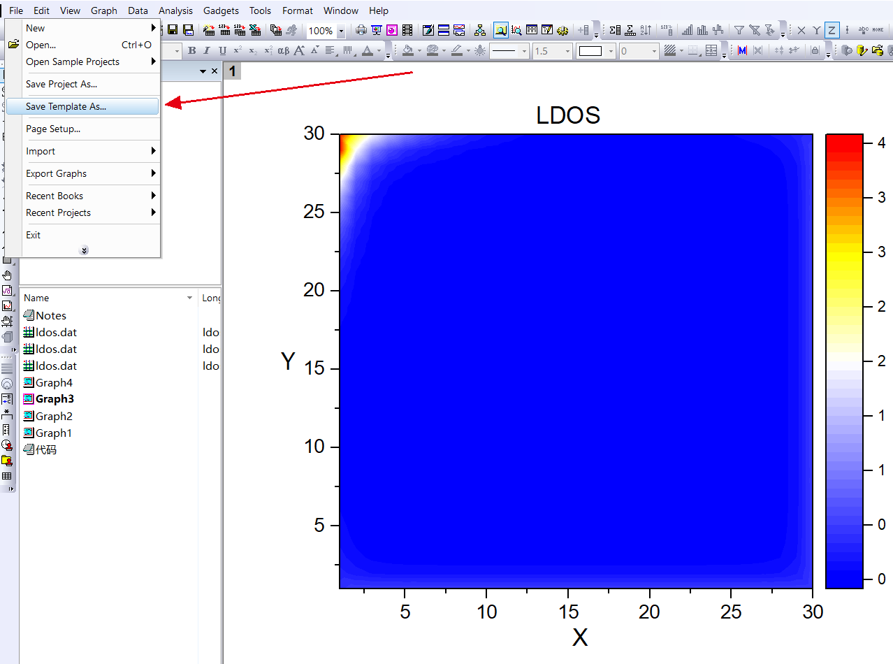
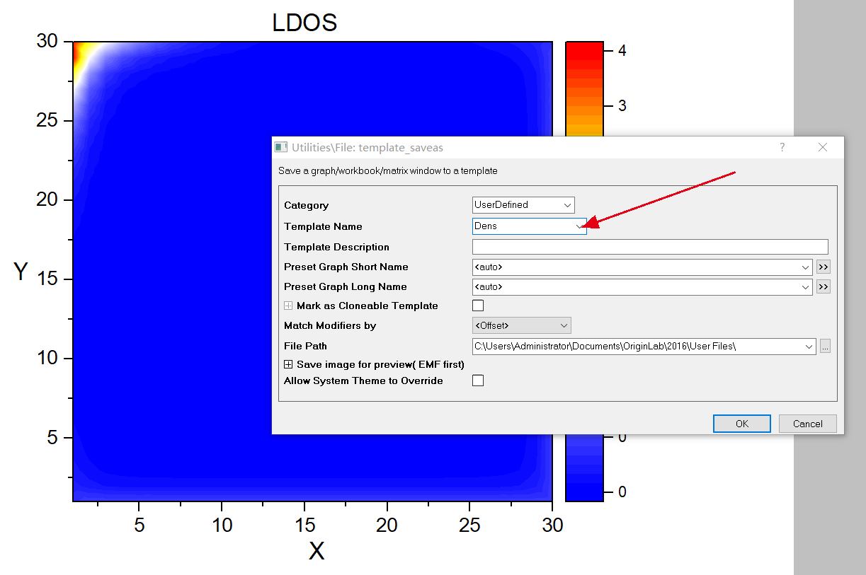
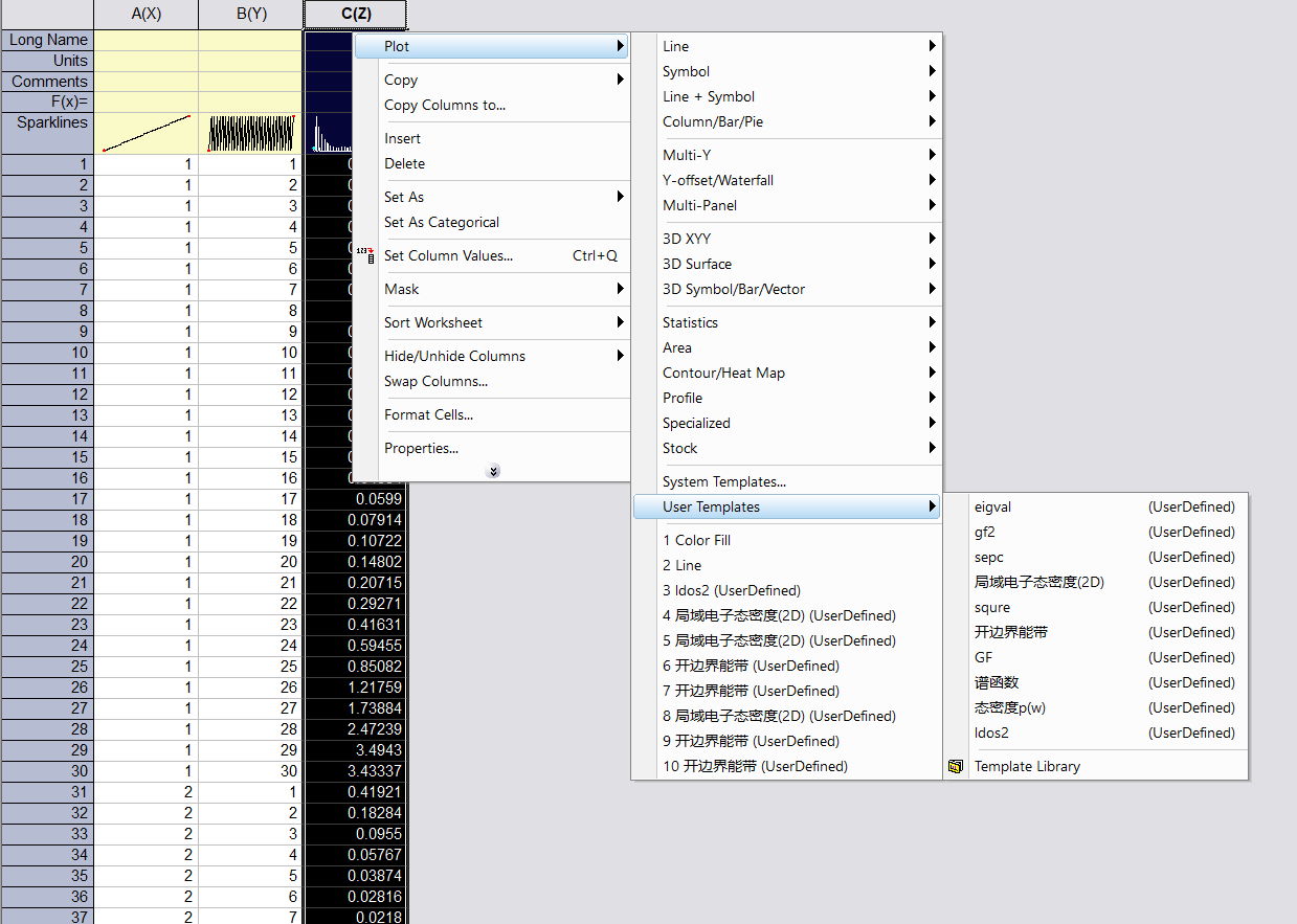
建立自己的作图模板
补充
批量编译执行Fortran程序
仅仅执行确定文件夹下的Fortran程序,再下一级目录中文件不会去执行1
2
3
4
5
6
7
8
9
10!/bin/sh
============ get the file name ===========
Folder="/home/yxli/te" #要批量编译哪个文件夹下面的Fortran
for file_name in ${Folder}/*.f90
do
temp_file=`basename $file_name .f90`
ifort -mkl $file_name -o $temp_file.out
./$temp_file.out & # 编译成功之后自动运行
done
rm *out # 删除编译后文件批量执行文件夹中所有的Fortran程序(文件夹中可以包含文件夹)
递归搜寻文件夹下面所有的Fortran文件
1 | !/bin/bash |
鉴于该网站分享的大都是学习笔记,作者水平有限,若发现有问题可以发邮件给我
- yxliphy@gmail.com
也非常欢迎喜欢分享的小伙伴投稿


欢迎关注公众号,有趣的内容也会在上面同步。 有密码的文章属于正在建设中或者没有通过验证的内容,若有需要可通过邮件联系。

![超导自由能泛函(Ginzburg–Landau)推导[非均匀配对]](/assets/images/SC/SC-Free.png)