虽然我经常利用Origin来作图,但是它的绘图样式现在看起来真的不是特别好看,包括作图的颜色还有一些作图的形式.这里就整理下我之前利用Julia画的一些图,我觉得它的样式还是很符合我的审美的.
密度分布
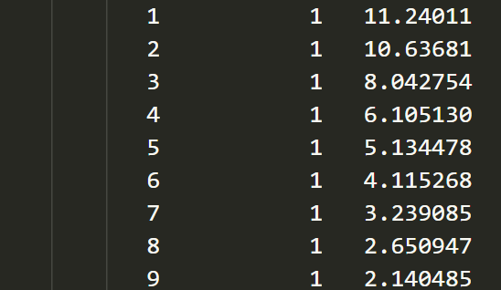
我这里的数据是用Fortran计算的,密度图的数据格式为$[x \quad y\quad z]$,在Julia中需要对这中格式的数据进行一定的操作,然后进行绘图.计算得出的数据格式如下
figure(figsize=(10,8)) # 画图大小
f = open("corner.dat") # 数据文件名
s = readdlm(f)
s = reshape(s,(convert(Int32,length(s)/3),3))
x = s[:,1]
y = s[:,2]
z = s[:,3]
a1 = scatter(x,y,z*20,c=z,edgecolors="b",cmap="Reds")
colorbar(a1) # 加入颜色条
xticks(0:5:maximum(x))
yticks(0:5:maximum(y))
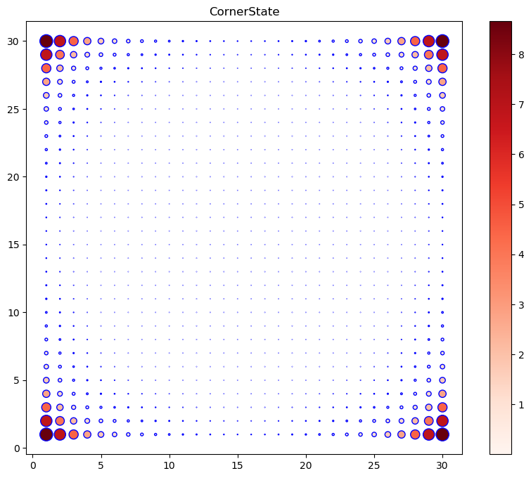
title("CornerState")
savefig("cor.eps",bbox_inches="tight",dpi=300) # 保存作图文件
子图
# ======================================================
figure(figsize=(14,5))
subplot(121)
f = open("op1.dat")
s = readdlm(f)
s = reshape(s,(convert(Int32,length(s)/3),3))
x = s[:,1]
y = s[:,2]
z = s[:,3]
a1 = scatter(x,y,z*5000,c=z,edgecolors="b",cmap="Reds")
colorbar(a1)
xticks(1:2:maximum(x))
yticks(1:2:maximum(y))
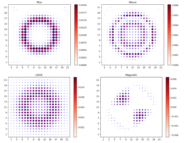
title("Plus")
# ----------------------------------------------
subplot(122)
f = open("op2.dat")
s = readdlm(f)
s = reshape(s,(convert(Int32,length(s)/3),3))
x = s[:,1]
y = s[:,2]
z = s[:,3]
a1 = scatter(x,y,z*10000,c=z,edgecolors="b",cmap="Reds")
colorbar(a1)
xticks(1:2:maximum(x))
yticks(1:2:maximum(y))
title("Minus")
savefig("op.png",bbox_inches="tight")
# ==========================================================================================
figure(figsize=(14,5))
subplot(121)
f = open("ldos.dat")
s = readdlm(f)
s = reshape(s,(convert(Int32,length(s)/3),3))
x = s[:,1]
y = s[:,2]
z = s[:,3]
a1 = scatter(x,y,z*5000,c=z,edgecolors="b",cmap="Reds")
colorbar(a1)
xticks(1:2:maximum(x))
yticks(1:2:maximum(y))
title("LDOS")
# ----------------------------------------------
subplot(122)
f = open("magnum.dat")
s = readdlm(f)
s = reshape(s,(convert(Int32,length(s)/3),3))
x = s[:,1]
y = s[:,2]
z = s[:,3]
a1 = scatter(x,y,z*10000,c=z,edgecolors="b",cmap="Reds")
colorbar(a1)
xticks(1:2:maximum(x))
yticks(1:2:maximum(y))
title("Magnetic")
savefig("ldos.eps",bbox_inches="tight")
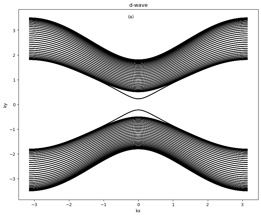
多曲线作图
通常在做cylinder结构的能带图时,其实就是在一张图上做出多条曲线,计算得到的数据结构如下
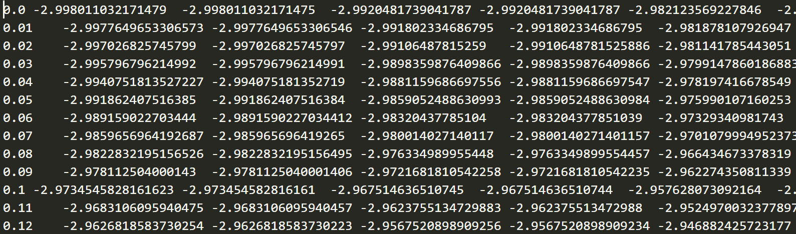
每一行代表一个固定$k_i$下的能量本征值
figure(figsize=(10,8))
f = open("engband.dat")
s = readdlm(f)
#s = reshape(s,(convert(Int32,length(s)/3),3))
p=plot(s[:,1],s[:,2:end],"black")
title("d-wave")
xlabel("kx")
ylabel("ky")
annotate("(a)", xy=(0,0), xytext=(-0.3, 3.5))
savefig("eband.eps",bbox_inches="tight",dpi=300)
close(f)
函数集成
上面的只是简单的展示了一下julia的作图功能,这里我将所有的内容整理成函数,这样只需要输入所要作图的文件名,即可以按照上面的样式进行图形绘制
using PyPlot,DelimitedFiles
# =======================================================
function density2D(file_name::String)
    # 2D density plot
    figure(figsize=(10,8))
    f = open(file_name)
    s = readdlm(f)
    s = reshape(s,(convert(Int32,length(s)/3),3))
    x = s[:,1]
    y = s[:,2]
    z = s[:,3]
    a1 = scatter(x,y,z*20,c=z,edgecolors="b",cmap="Reds")
    colorbar(a1)
    xticks(0:10:maximum(x))
    yticks(0:10:maximum(y))
    title("CornerState")
    savefig("cor.eps",bbox_inches="tight",dpi=300)
end
# --------------------------------------------------------
function cylinder(file_name::String)
    # topological cylinder gemoetry band structure
    figure(figsize=(10,8))
    f = open(file_name)
    s = readdlm(f)
    #s = reshape(s,(convert(Int32,length(s)/3),3))
    #p=plot(s[:,1],s[:,2:end],"black")
    p=plot(s[:,1],s[:,2:end])
    title("cylinder-geometry")
    xlabel("kx")
    ylabel("ky")
    #annotate("(a)", xy=(0,0), xytext=(-0.3, 3.5))
    savefig("eband.eps",bbox_inches="tight",dpi=300)
    close(f)
end
从整体上来看,Julia的绘图功能确实没有Python那么齐全,很多细节的地方还有一些标签的样式也无法精确的控制,不过相信这会发展的越来越好的.
公众号
相关内容均会在公众号进行同步,若对该Blog感兴趣,欢迎关注微信公众号。

|
yxli406@gmail.com |