PythonTB学习笔记
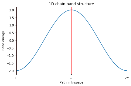
简单一维模型求解
1 | #!/usr/bin/env python |
Path in 1D BZ defined by nodes at [0. 0.5 1. ]
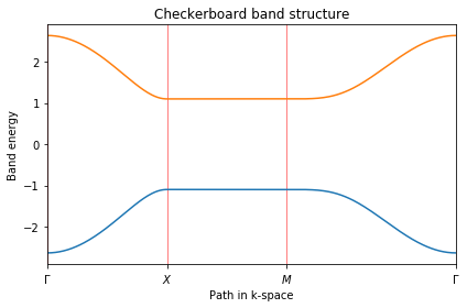
二维模型求解
1 | #!/usr/bin/env python |
----- k_path report begin ----------
real-space lattice vectors
 [[1. 0.]
 [0. 1.]]
k-space metric tensor
 [[1. 0.]
 [0. 1.]]
internal coordinates of nodes
 [[0.  0. ]
 [0.  0.5]
 [0.5 0.5]
 [0.  0. ]]
reciprocal-space lattice vectors
 [[1. 0.]
 [0. 1.]]
cartesian coordinates of nodes
 [[0.  0. ]
 [0.  0.5]
 [0.5 0.5]
 [0.  0. ]]
list of segments:
  length =     0.5  from  [0. 0.]  to  [0.  0.5]
  length =     0.5  from  [0.  0.5]  to  [0.5 0.5]
  length = 0.70711  from  [0.5 0.5]  to  [0. 0.]
node distance list: [0.      0.5     1.      1.70711]
node index list:    [  0  88 176 300]
----- k_path report end ------------

---------------------------------------
starting calculation
---------------------------------------
Calculating bands...
Plotting bandstructure...
Done.
1 | #!/usr/bin/env python |
 Path in 1D BZ defined by nodes at [-0.5  0.   0.5]

---------------------------------------
starting calculation
---------------------------------------
Calculating bands...
Plotting bandstructure...
Done.
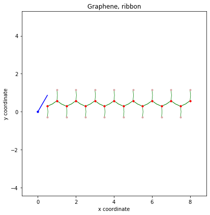
从能带的计算结果就可以看到,在构建模型的时候,每个元胞中是有两个轨道的,如果认为每个轨道来自不同的原子的话,也就是每个元胞中都是由2个原子的
1 | #!/usr/bin/env python |
---------------------------------------
starting calculation
---------------------------------------
Calculating bands...

Band energies

Done.
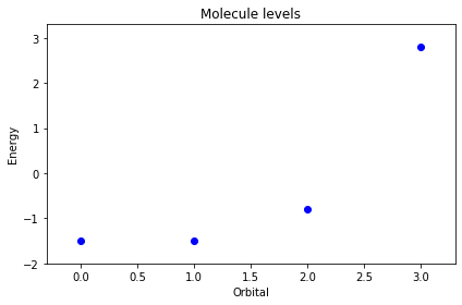
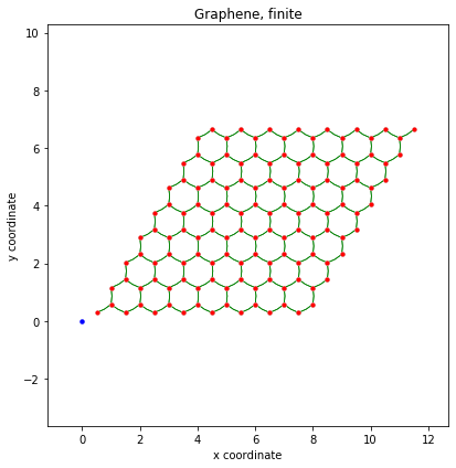
从计算结果也可以清楚的看到,一个分子中,也可以认为是一个元胞中有4个TB轨道,所以对于单分子进行求解之后,也就只有4个能量本征值
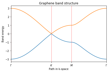
Graphene model
1 | #!/usr/bin/env python |
----- k_path report begin ----------
real-space lattice vectors
 [[1.      0.     ]
 [0.5     0.86603]]
k-space metric tensor
 [[ 1.33333 -0.66667]
 [-0.66667  1.33333]]
internal coordinates of nodes
 [[0.      0.     ]
 [0.66667 0.33333]
 [0.5     0.5    ]
 [0.      0.     ]]
reciprocal-space lattice vectors
 [[ 1.      -0.57735]
 [ 0.       1.1547 ]]
cartesian coordinates of nodes
 [[0.      0.     ]
 [0.66667 0.     ]
 [0.5     0.28868]
 [0.      0.     ]]
list of segments:
  length = 0.66667  from  [0. 0.]  to  [0.66667 0.33333]
  length = 0.33333  from  [0.66667 0.33333]  to  [0.5 0.5]
  length = 0.57735  from  [0.5 0.5]  to  [0. 0.]
node distance list: [0.      0.66667 1.      1.57735]
node index list:    [  0  51  76 120]
----- k_path report end ------------

---------------------------------------
starting calculation
---------------------------------------
Calculating bands...
Done.
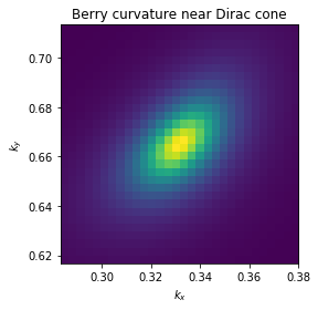
Berry phase around Dirac cone in graphene
1 | #!/usr/bin/env python |
Berry phase along circle with radius:  0.05
  centered at k-point:  [0.33333333 0.66666667]
  for band 0 equals    :  2.068204018990522
  for band 1 equals    :  -2.068204018990522
  for both bands equals:  3.469446951953614e-17

Berry flux on square patch with length:  0.1
  centered at k-point:  [0.33333333 0.66666667]
  for band 0 equals    :  2.179216480131516
  for band 1 equals    :  -2.1792164801315166
  for both bands equals:  3.308776163370093e-16

Done.
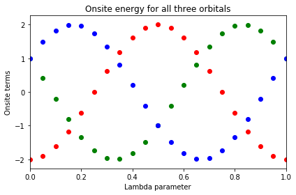
One-dimensional cycle of 1D tight-binding model
1 | #!/usr/bin/env python |
Berry flux in k-lambda space:  -6.283185307179586
Done.
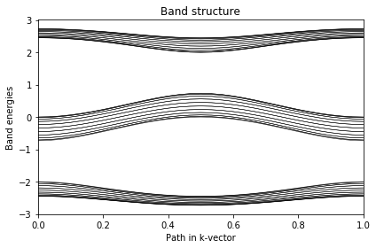
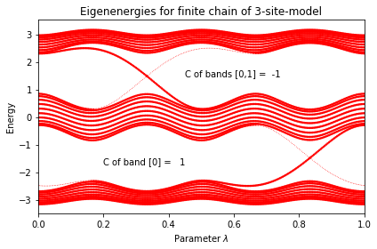
One-dimensional cycle on a finite 1D chain
1 | #!/usr/bin/env python |
Chern numbers for rising fillings
  Band  0     =  1.00
  Bands 0,1   = -1.00
  Bands 0,1,2 = -0.00

Chern numbers for individual bands
  Band  0 =  1.00
  Band  1 = -2.00
  Band  2 =  1.00

Done.
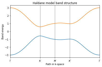
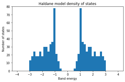
Haldane model
1 | #!/usr/bin/env python |
----- k_path report begin ----------
real-space lattice vectors
 [[1.      0.     ]
 [0.5     0.86603]]
k-space metric tensor
 [[ 1.33333 -0.66667]
 [-0.66667  1.33333]]
internal coordinates of nodes
 [[0.      0.     ]
 [0.66667 0.33333]
 [0.5     0.5    ]
 [0.33333 0.66667]
 [0.      0.     ]]
reciprocal-space lattice vectors
 [[ 1.      -0.57735]
 [ 0.       1.1547 ]]
cartesian coordinates of nodes
 [[0.      0.     ]
 [0.66667 0.     ]
 [0.5     0.28868]
 [0.33333 0.57735]
 [0.      0.     ]]
list of segments:
  length = 0.66667  from  [0. 0.]  to  [0.66667 0.33333]
  length = 0.33333  from  [0.66667 0.33333]  to  [0.5 0.5]
  length = 0.33333  from  [0.5 0.5]  to  [0.33333 0.66667]
  length = 0.66667  from  [0.33333 0.66667]  to  [0. 0.]
node distance list: [0.      0.66667 1.      1.33333 2.     ]
node index list:    [  0  33  50  67 100]
----- k_path report end ------------


---------------------------------------
starting DOS calculation
---------------------------------------
Calculating DOS...
Plotting DOS...
Done.
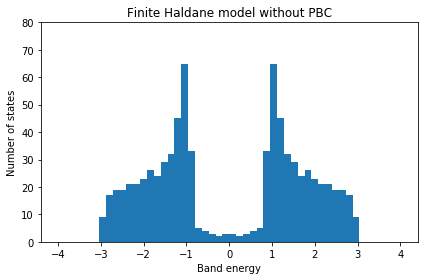
Finite Haldane model
1 | #!/usr/bin/env python |
Done.

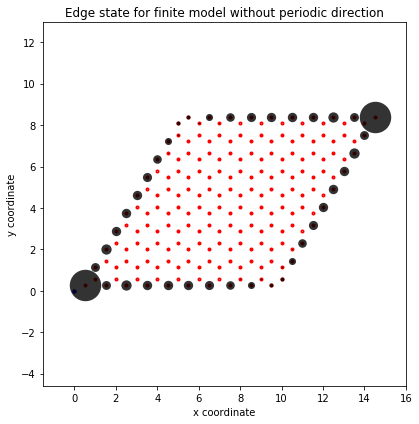
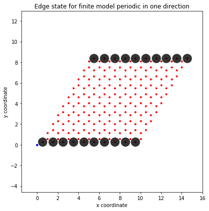
Edge states
1 | #!/usr/bin/env python |
Done.
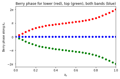
Berry phases in Haldane model
1 | #!/usr/bin/env python |
Using approach #1
 Berry flux=  -6.283185307179586
Using approach #2
 Berry flux=  -6.283185307179586
Done.
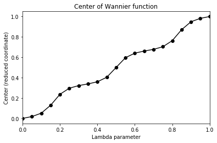
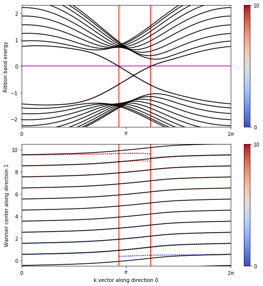
Hybrid Wannier centers in Haldane model
1 | #!/usr/bin/env python |
Done.
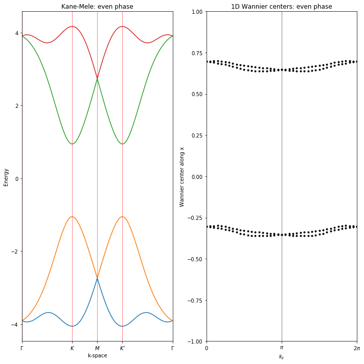
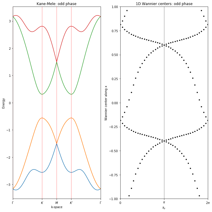
Kane-Mele model using spinor features
1 | #!/usr/bin/env python |
Done.
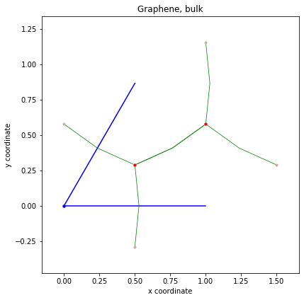
Visualization example
1 | #!/usr/bin/env python |
Done.
鉴于该网站分享的大都是学习笔记,作者水平有限,若发现有问题可以发邮件给我
- yxliphy@gmail.com
也非常欢迎喜欢分享的小伙伴投稿
本博客所有文章除特别声明外,均采用 CC BY-NC-SA 4.0 许可协议。转载请注明来源 Yu-Xuan's Blog!


相关推荐

2020-07-01
两种方法计算Chern Number
计算Chern数是最初学习拓扑物理都会遇到的问题,正好在假期空闲的时候自己学习了一下Chern数的数值计算方法,在博客上记录一下希望可以帮助到别人。 具体的计算方法和细节就不在这里说明了,只...

2020-08-10
超大型系数矩阵对角化
最近在进行一些三维实空间中系统性质的研究,利用紧束缚束缚模型,当三个方向都取开边界时,矩阵会变的非常大,组里的服务器完全不能计算,所以只好寻找一些替代的方法。首先哈密顿量是个大型系数矩阵,这个时...
2020-09-14
Julia,Python,Fortran,Mathematica循环计算速度比较
在平时进行数值计算时,我经常会遇到的两种比较消耗时间计算,其一是对大型矩阵的对角化问题,这是在对哈密顿量厄密矩阵求解本征问题时经常遇到的;另外一个就是循环计算了,这个结构在动量空间计算体系格林函...
评论
公告

欢迎关注公众号,有趣的内容也会在上面同步。 有密码的文章属于正在建设中或者没有通过验证的内容,若有需要可通过邮件联系。