因为对格林函数很熟悉,在看文章的时候也有遇到计算体系准粒子干涉的文章,最后只明白可以通过干涉的分布样式来判断不同费米面之间的散射问题,从而来确定体系费米面上的一些性质,还有就是这些干涉的图案还是很好看的,所以一直也就想自己动手去算一下,这里我就想从一个很简单的例子来学习一些如何编程计算准粒子干涉的图样,同时也算是对文章的进一步理解.
{:.info}

这里主要是想重复Quasiparticle scattering interference in superconducting iron pnictides这篇文章中的主要结果,因为自己就是搞超导方向的(好吧,我承认我对超导其实理解并没有很深入),所以就利用这篇铁基超导的准粒子干涉计算来练练手.
{:.warning}

Fortran

1
2
3
4
5
6
7
8
9
10
11
12
13
14
15
16
17
18
19
20
21
22
23
24
25
26
27
28
29
30
31
32
33
34
35
36
37
38
39
40
41
42
43
44
45
46
47
48
49
50
51
52
53
54
55
56
57
58
59
60
61
62
63
64
65
66
67
68
69
70
71
72
73
74
75
76
77
78
79
80
81
82
83
84
85
86
87
88
89
90
91
92
93
94
95
96
97
98
99
100
101
102
103
104
105
106
107
108
109
110
111
112
113
114
115
116
117
118
119
120
121
122
123
124
125
126
127
128
129
130
131
132
133
134
135
136
137
138
139
140
141
142
143
144
145
146
147
148
149
150
151
152
153
154
155
156
157
158
159
160
161
162
163
164
165
166
167
168
169
170
171
172
173
174
175
176
177
178
179
180
181
    module pub
implicit none
integer N,ne,kn
parameter(N = 4,ne = 100,kn = 200)
real,parameter::pi = 3.14159265358
complex,parameter::im = (0.0,1.0)
complex ham(N,N)
complex gf0(N,N) ! bare green's function
complex tmat(N,N) ! T-matrix
complex::V(N,N) = 0.0
real t1,t2,t3,t4,del0,mu,eta,v0
!-----Package needed----------
integer info
end module pub
!=================================================================
program sol
use pub
t1 = -1
t2 = 1.3
t3 = -0.85
t4 = -0.85
del0 = 0.1
mu = 1.54
v0 = 0.4
eta = 0.05 ! quasiparticle dumping
!-------------
! impurity matrix
V(1,1) = V0
V(2,2) = -V0
V(3,3) = V0
V(4,4) = -V0
!-------------
! call main(0.07)
call spectrum(0.07)
stop
end program sol
!==================================================================
subroutine spectrum(omg)
! 纯净系统的谱函数计算
use pub
integer m1,m2
real kx,ky,omg
open(11,file="spec.dat")
do m1 = -kn,kn
do m2 = -kn,kn
kx = m1*pi/kn
ky = m2*pi/kn
call gf_clean(kx,ky,omg)
write(11,*)kx/pi,ky/pi,-aimag((gf0(1,1) + gf0(3,3))/pi)
end do
end do
close(11)
return
end subroutine spectrum
!==================================================================
subroutine main(omg)
use pub
integer m1,m2,m3,m4
real qx,qy,kx,ky,omg
complex gf1(N,N),gf2(N,N),re1,rho0
call scmat(omg) ! 得到 T 矩阵
open(10,file='scat.dat')
do m1 = -ne,ne
qx = m1*pi/ne
do m2 = -ne,ne
qy = m2*pi/ne
rho0 = 0
do m3 = -ne,ne
kx = pi*m3/ne
do m4 = -ne,ne
ky = pi*m4/ne
call gf_clean(kx,ky,omg)
gf1 = gf0
call gf_clean(kx + qx,ky + qy,omg)
gf2 =gf0
gf2 = matmul(matmul(gf1,tmat),gf2) ! 计算杂质系统的格林函数
re1 = gf2(1,1) - conjg(gf2(1,1)) + gf2(3,3) - conjg(gf2(3,3)) ! 态密度计算(这里需要具体参考文章,或者是你想计算什么态密度)
rho0 = rho0 + re1*(1.0/ne)**2
end do
end do
rho0 = rho0/(2.0*pi)**3*im
write(10,*)qx/pi,qy/pi,real(rho0)
end do
end do
close(10)
return
end subroutine main
!==================================================================
subroutine scmat(omg)
! 加入杂质后利用杂质矩阵和纯净系统的GF计算散射T-matrix
use pub
real kx,ky,omg
integer m1,m2,m3,m4
complex ga(N,N),temp1(N,N),temp2(N,N) ! green's function FT 后的结果
! green's function 傅里叶变化
do m1 = -ne,ne
do m2 = -ne,ne
kx = m1*pi/ne
ky = m2*pi/ne
call matset(kx,ky)
call gf_clean(kx,ky,omg)
do m3 = 1,N
do m4 = 1,N
ga(m3,m4) = ga(m3,m4) + gf0(m3,m4)*1.0/ne
end do
end do
end do
end do
ga = ga/(2.0*pi)**2
!-----------------------------------------------
! T-matrix compute
! tmat = matmul(1 - matmul(V,ga),V)

temp1 = 1 - matmul(V,ga)
call inv(temp1,temp2)
tmat = matmul(temp2,V)
return
end subroutine scmat
!==========================================================================
subroutine gf_clean(kx,ky,omg)
! 未加杂质时的格林函数
use pub
real kx,ky,omg
integer m1,m2
complex::temp1(N,N) = 0
call matset(kx,ky)
do m1 = 1,N
do m2 = 1,N
temp1(m1,m2) = omg - im*eta - ham(m1,m2)
end do
end do
call inv(temp1,gf0) ! 求逆的结果保存在gf0中,由哈密顿量得到其对应的格林函数
return
end subroutine gf_clean
!==========================================================================
subroutine matset(kx,ky)
use pub
real kx,ky
ham = 0

ham(1,1) = (-2*t1*cos(kx) - 2*t2*cos(ky) - 4*t3*cos(kx)*cos(ky)) - mu
ham(2,2) = -(-2*t1*cos(kx) - 2*t2*cos(ky) - 4*t3*cos(kx)*cos(ky)) + mu
ham(3,3) = (-2*t1*cos(ky)-2*t2*cos(kx)-4*t3*cos(kx)*cos(ky))-mu
ham(4,4) = -(-2*t1*cos(ky)-2*t2*cos(kx)-4*t3*cos(kx)*cos(ky)) + mu

ham(1,2) = del0*cos(kx)*cos(ky)
ham(2,1) = del0*cos(kx)*cos(ky)
ham(1,3) = -4*t4*sin(kx)*sin(ky)
ham(3,1) = -4*t4*sin(kx)*sin(ky)
ham(1,4) = 0.0
ham(4,1) = 0.0

ham(2,3) = 0.0
ham(3,2) = 0.0
ham(2,4) = -(-4*t4*sin(kx)*sin(ky))
ham(4,2) = -(-4*t4*sin(kx)*sin(ky))

ham(3,4) = del0*cos(kx)*cos(ky)
ham(4,3) = del0*cos(kx)*cos(ky)

return
end subroutine matset
!=======================矩阵求逆====================================
subroutine inv(matin,matout)
use pub
complex,intent(in) :: matin(N,N)
complex:: matout(size(matin,1),size(matin,2))
real:: work2(size(matin,1)) ! work2 array for LAPACK
integer::ipiv(size(matin,1)) ! pivot indices
! Store matin in matout to prevent it from being overwritten by LAPACK
matout = matin
! SGETRF computes an LU factorization of a general M-by-N matrix A
! using partial pivoting with row interchanges.
call CGETRF(N,N,matout,N,ipiv,info)
if (info.ne.0) stop 'Matrix is numerically singular!'
! SGETRI computes the inverse of a matrix using the LU factorization
! computed by SGETRF.
call CGETRI(N,matout,N,ipiv,work2,N,info)
if (info.ne.0) stop 'Matrix inversion failed!'
return
end subroutine inv

把文章仔细读过之后,再利用那些公式写出上面Fortran的程序并不难,但是上面的计算中有一个问题,那就是所有的执行都是串行的,不管我的服务器有多厉害还,cpu利用率也就只是100%,所以计算速度比较慢,虽然Fortran也是可以并行的,但是之前在看的时候,发现如果想用Fortran并行,需要去学习一下mpi或者openmpi,而且还必须在服务器上安装好这个玩意才可以,想想就觉得这是一个大工程,不过自己又正好熟悉Julia,这个号称速度比肩Fortran,灵活性比肩python的编程这一点我是已经体验过了,速度上的优势还没体现出来,正好在这里借这个文章来利用Julia的多线程计算一下准粒子干涉,体现一下速度优势.

Julia

1
2
3
4
5
6
7
8
9
10
11
12
13
14
15
16
17
18
19
20
21
22
23
24
25
26
27
28
29
30
31
32
33
34
35
36
37
38
39
40
41
42
43
44
45
46
47
48
49
50
51
52
53
54
55
56
57
58
59
60
61
62
63
64
65
66
67
68
69
70
71
72
73
74
75
76
77
78
79
80
81
82
83
using ProgressMeter
using Distributed
using DelimitedFiles
@everywhere using SharedArrays, LinearAlgebra #利用@everywhere红之后,表示在启动的所有线程上都分享这个using
#using PyPlot

# println(nprocs()) # 当前现有的线程数目
addprocs(15 - nprocs()) # 设置启动的线程数目
# println("Running ",nprocs()," processes") # 输出当前启动的线程数目

function hamset(kx::Float64, ky::Float64)::Matrix{Float64}
# 构建系统哈密顿量
Ex = -2 * t1 * cos(kx) - 2*t2*cos(ky) - 4*t3*cos(kx)*cos(ky)
Ey = -2*t1*cos(ky) - 2*t2*cos(kx) - 4*t3*cos(kx)*cos(ky)
Exy = -4*t4*sin(kx)*sin(ky)
del = d0*cos(kx)*cos(ky)
return [
[(Ex - mu) del Exy 0 ]
[ del (-Ex + mu) 0 -Exy]
[Exy 0 (Ey - mu) del ]
[0 -Exy del (-Ey + mu)]]
end
# ================================================================
function generateG(N)::Array{Matrix{ComplexF64}}
a = -pi + pi/N : 2*pi/N : (pi - pi / N + 0.00001 )
wI4 = (omega + im * delta).* I4
[inv( wI4 - hamset(kx, ky)) for kx=a, ky=a]
end
# ================================================================
@everywhere function rho(qx, qy, G0, TG0, st, N)::ComplexF64
# 因为在之后的多线程计算的时候就是要把这个函数分发到不同的线程上面,所以利用宏@everywhere来实现将这个函数广播到所有
# 的线程中
result = 0.0
for kx in 1:st:N, ky in 1:st:N
kpx = (kx + qx - 1 + N) % N + 1
kpy = (ky + qy - 1 + N) % N + 1
Gkkp = G0[kx, ky] * TG0[kpx, kpy]
Gkpk = G0[kpx, kpy] * TG0[kx, ky]
result += Gkkp[1,1] - conj(Gkpk[1, 1]) + Gkkp[3, 3] -conj(Gkpk[3,3])
# print(result, ' ')
end
return real(result * im)
end
# =====================================================================
println("preparing G^0 etc ...")

omega = -0.13
V0 = 0.4
N = 400 # 画图的格点数
M = 200 # 积分时用的格点数,可以比画图用的格点少几倍
d0 = 0.1
mu = 1.25
delta = 0.005
st = convert(Int, (N / M))
(t1, t2, t3, t4) = (-1, 1.3, -0.85, -0.85)
I2 = zeros(Float64,2,2) #构建单位矩阵
I4 = zeros(Float64,2,2)
V = kron(I2, (V0.* I2))

G0 = generateG(N)
Gamma0 = sum(G0[1:st:N, 1:st:N]) / (M^2)
T = inv(I4 - V*Gamma0) * V
TG0 = [T * g for g in G0]

println("Start calculation")

offset = convert(Int, N/2) # 用来把布里渊区中心移动到图中央(将一个值转换成int整形)
final = SharedArray(zeros(N, N)) # 初始化一个矩阵,让它来接受所有并行线程的结果
@time @sync @distributed for qx in 1:N # 只在这里开了多线程,并行计算像素点
# @time来计算程序执行时间 @distributed 用来将循环分发到不同的线程进行计算,可以节省时间
for qy in 1:N
final[qx, qy] = rho(qx-offset, qy-offset, G0, TG0, st, N)
end
end

filename = "result.dat"
f1 = open(filename,"w")
# code for plot
#PyPlot.set_cmap("gray_r")
#imsave(filename * ".png", -final)
for qx in 1:N,qy in 1:N
writedlm(f1,[qx*pi/N qy*pi/N final[qx,qy]])
end

总结

从速度上来说确实这里Julia的优势是很明显的,因为这里开了16个线程同时计算,在相同的参数下计算,Julia很快就可以计算完成,而Fortran的话,估计要算很久,因为是单线程串行,所以速度是相当的慢,而且这里在计算的时候因为嵌套的循环比较多,这就导致这种写法下,Fortran的计算速度真的就是很慢了,所以在这里Julia是获胜了.最重要的是,利用julia进行并行多线程的时候,并不需要很复杂的东西,只需要掌握简单的知识就好了,它用到的额外的几个库,用很简单的命令增加库就可以,相比较与Fortran来说简直就是态方便了.

Julia + Gnuplot

虽然Julia也可以绘图,但是使用起来始终没有Gnupltot那么方便,这里可以通过调整一下程序,让得到的数据结果可以方便的利用Gnuplot来绘图

1
2
3
4
5
6
7
8
9
10
11
12
13
14
file = "result"
form = ".dat"
filename = join([file,1,form])
f1 = open(filename,"w")
# code for plot
#PyPlot.set_cmap("gray_r")
#imsave(filename * ".png", -final)
for qx in 1:N
for qy in 1:N
writedlm(f1,[qx*pi/N qy*pi/N final[qx,qy]])
end
writedlm(f1," ")
end
close(f1)

经过这样的修改之后,首先filename = join([file,1,form])可以实现批量命名文件,只要修改其中的第二个参数就可以,在for循环中加入writedlm(f1," ")是为了让内层循环计算一次之后,数据之间加入一个空行,这是为了配合Gnuplot绘图.
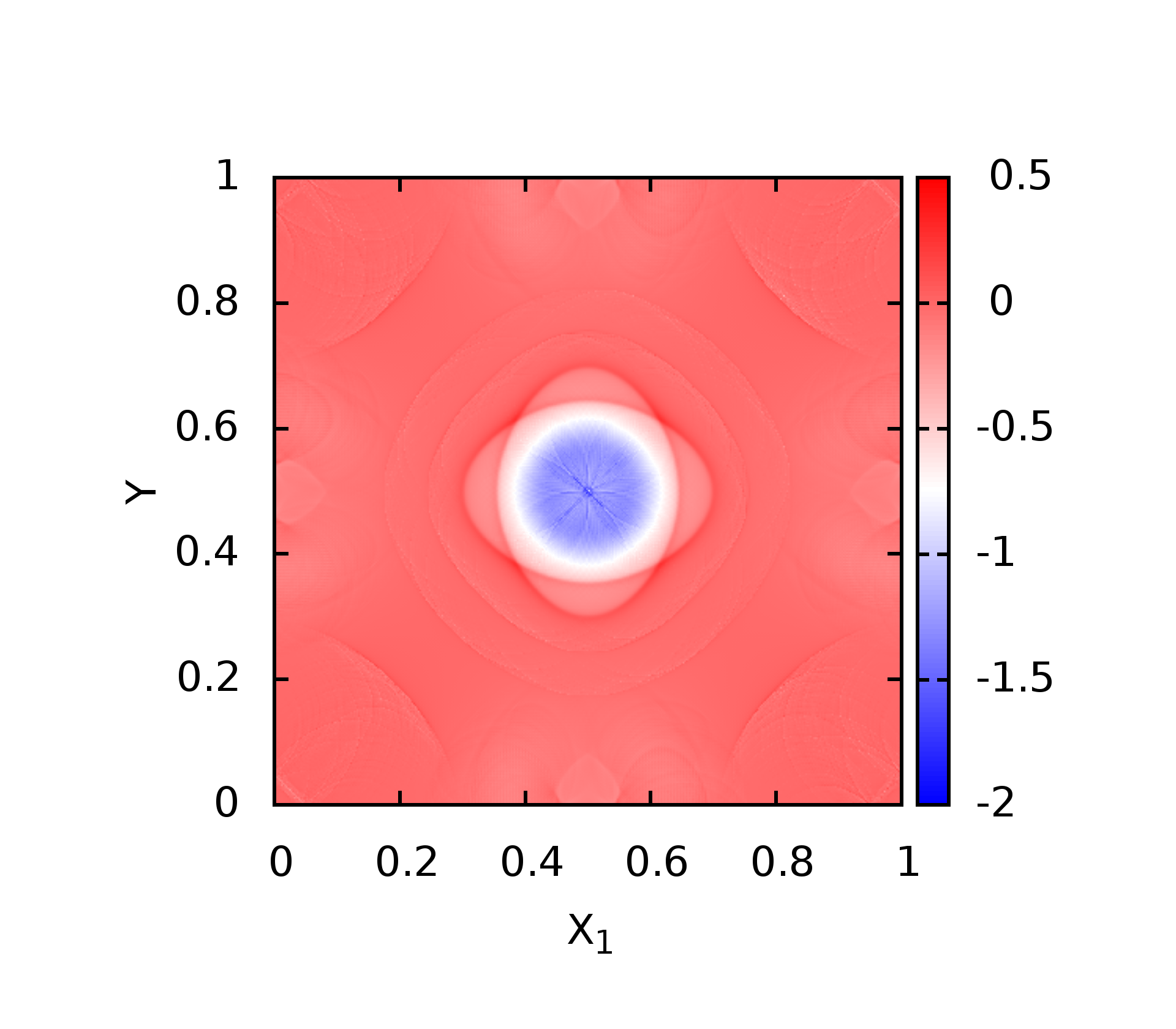
gnuplot 密度图

绘图模板如下

1
2
3
4
5
6
7
8
9
10
11
12
13
14
15
16
17
18
19
20
21
22
23
24
25
26
27
28
29
set encoding iso_8859_1
#set terminal postscript enhanced color
#set output 'arc_r.eps'
#set terminal pngcairo truecolor enhanced font ",50" size 1920, 1680
set terminal png truecolor enhanced font ",50" size 1920, 1680
set output 'density.png'
#set palette defined ( -10 "#194eff", 0 "white", 10 "red" )
set palette defined ( -10 "blue", 0 "white", 10 "red" )
#set palette rgbformulae 33,13,10
unset ztics
unset key
set pm3d
set border lw 6
set size ratio -1
set view map
set xtics
set ytics
#set xlabel "K_1 (1/{\305})"
set xlabel "k_x"
#set ylabel "K_2 (1/{\305})"
set ylabel "k_y"
set ylabel offset 1, 0
set colorbox
set xrange [0:1]
set yrange [0:1]
set pm3d interpolate 4,4
#splot 'wavenorm.dat' u 1:2:3 w pm3d
splot 'result1.dat' u 1:2:3 w pm3d

png

公众号

相关内容均会在公众号进行同步,若对该Blog感兴趣,欢迎关注微信公众号。
{:.info}

QR Code

Email

yxliphy@gmail.com