&TB_FILE Hrfile = 'wannier90_hr.dat' Package = 'VASP'! obtained from VASP, it could be 'VASP', 'QE', 'Wien2k', 'OpenMx' /
LATTICE Angstrom -2.069 -3.5836140.000000! crystal lattice information 2.069 -3.5836140.000000 0.0002.3890759.546667
ATOM_POSITIONS 5! number of atoms for projectors Direct! Direct or Cartisen coordinate Bi 0.39900.39900.6970 Bi 0.60100.60100.3030 Se 0.00000.00000.5000 Se 0.20600.20600.1180 Se 0.79400.79400.8820
PROJECTORS 33333! number of projectors Bi px py pz ! projectors Bi px py pz Se px py pz Se px py pz Se px py pz
SURFACE ! Specify surface with two vectors, see doc 100 010
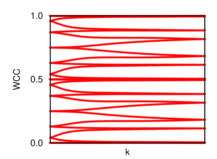
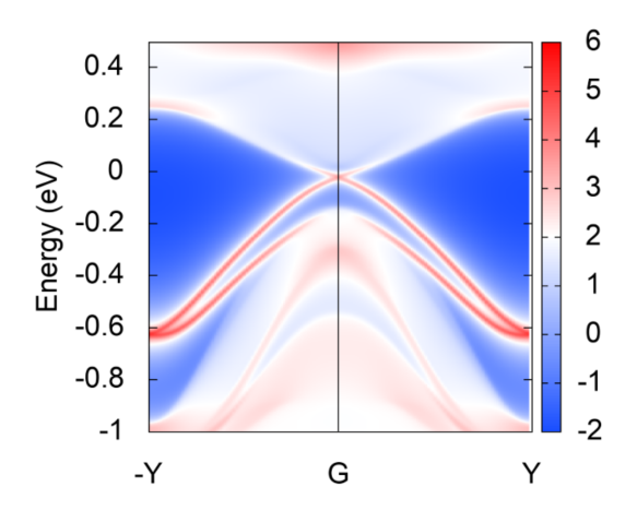
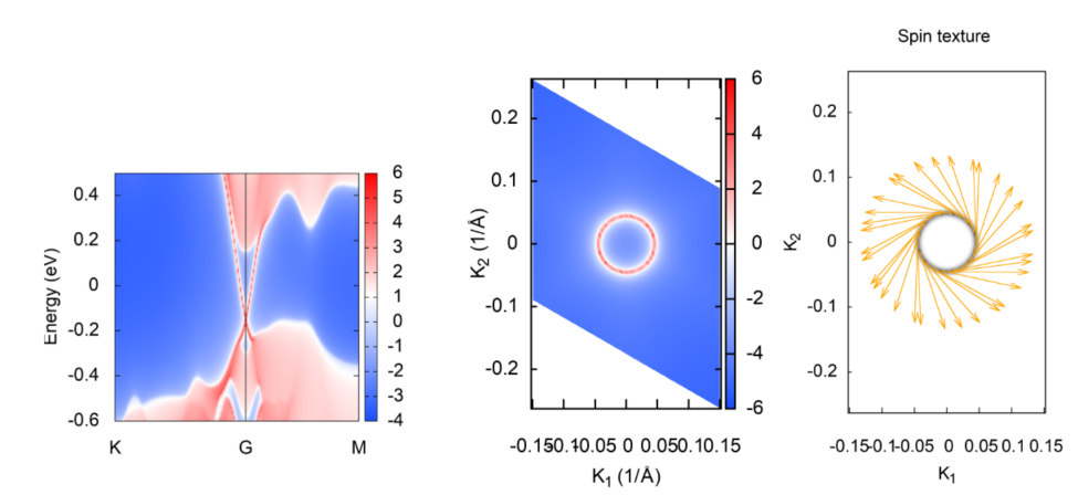
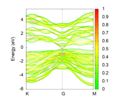
!> bulk band structure calculation flag &CONTROL BulkBand_calc = T BulkBand_points_calc = T DOS_calc = T SlabBand_calc = T SlabBandWaveFunc_calc = T SlabBand_plane_calc = T WireBand_calc = T SlabSS_calc = T SlabArc_calc = T SlabQPI_calc = T Z2_3D_calc = T SlabSpintexture_calc = T Wanniercenter_calc = T /
&SYSTEM NSLAB = 4! for thin film system NSLAB1= 2! nanowire system NSLAB2= 2! nanowire system NumOccupied = 18! NumOccupied SOC = 1! soc E_FERMI = 4.4195! e-fermi, a global shift of the energy levels surf_onsite= 0.0! surf_onsite /
&PARAMETERS Eta_Arc = 0.001! infinite small value, like brodening E_arc = 0.0! energy level for contour plot of spectrum OmegaNum = 400! omega number OmegaMin = -0.6! energy interval OmegaMax = 0.5! energy interval Nk1 = 10! number k points odd number would be better Nk2 = 10! number k points odd number would be better Nk3 = 10! number k points odd number would be better NP = 1! number of principle layers Gap_threshold = 0.01! threshold for FindNodes_calc output /
KPATH_BULK ! k point path 4! number of k line only for bulk band G 0.000000.000000.0000 Z 0.000000.000000.5000 Z 0.000000.000000.5000 F 0.500000.500000.0000 F 0.500000.500000.0000 G 0.000000.000000.0000 G 0.000000.000000.0000 L 0.500000.000000.0000
KPATH_SLAB 2! numker of k line for 2D case K 0.330.67 G 0.00.0! k path for 2D case G 0.00.0 M 0.50.5
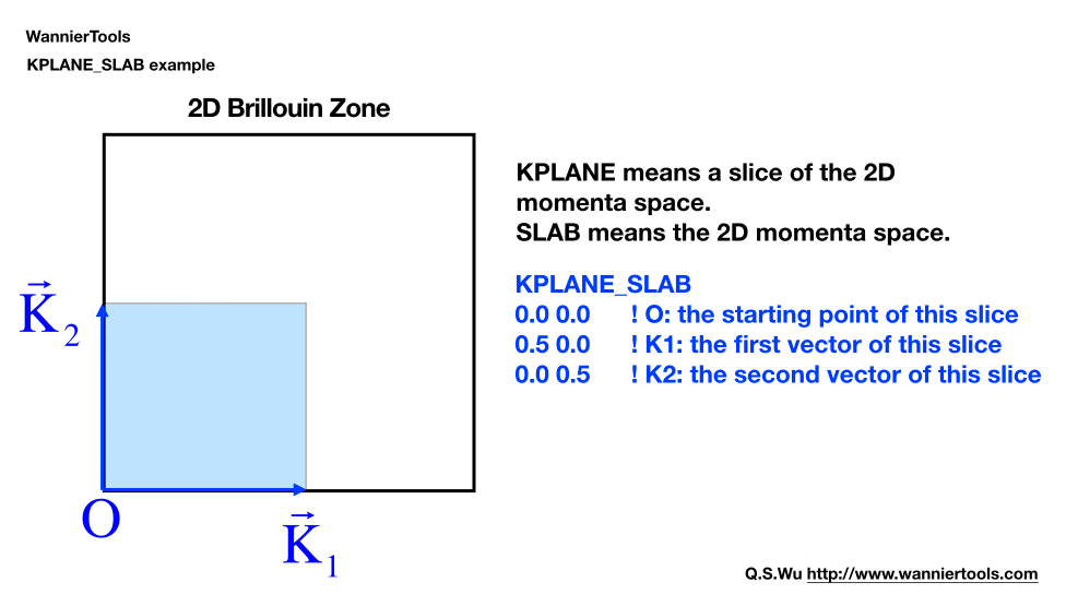
KPLANE_SLAB -0.1 -0.1! Original point for 2D k plane 0.20.0! The first vector to define 2D k plane 0.00.2! The second vector to define 2D k plane for arc plots
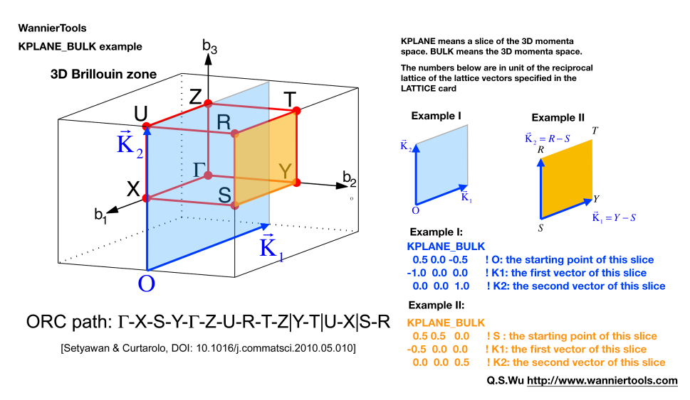
KPLANE_BULK 0.000.000.50! Original point for 3D k plane 1.000.000.00! The first vector to define 3d k space plane 0.000.500.00! The second vector to define 3d k space plane
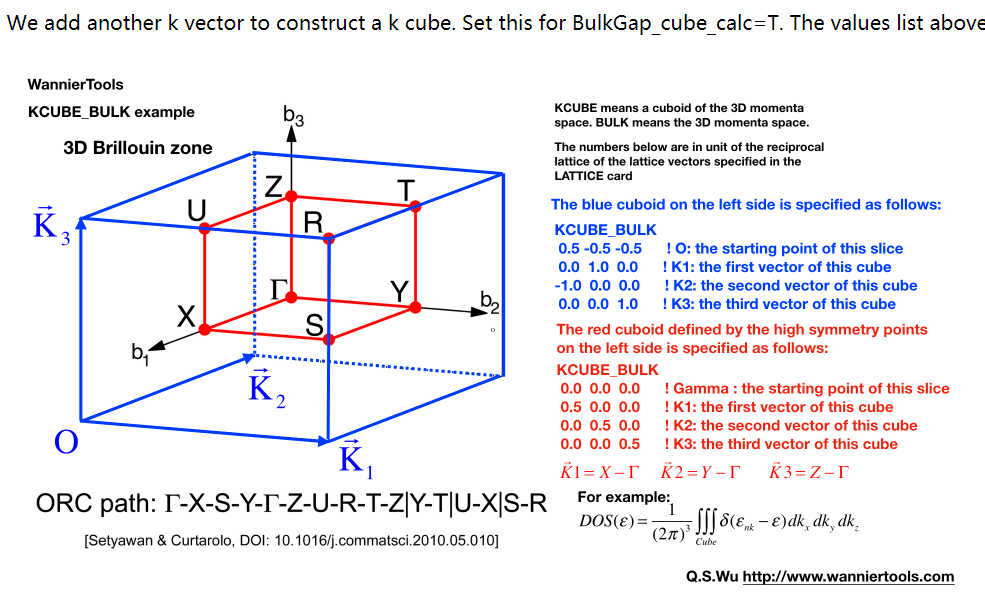
KCUBE_BULK -0.50 -0.50 -0.50! Original point for 3D k plane 1.000.000.00! The first vector to define 3d k space plane 0.001.000.00! The second vector to define 3d k space plane 0.000.001.00! The third vector to define 3d k cube
&TB_FILE ! 输入控制文件中共有4个这样的名字 TB_FILE, SYSTEM, CONTROL, PARAMETERS,分别用来控制不同内容 Hrfile = 'wannier90_hr.dat'! 紧束缚哈密顿量的位置 Package = 'VASP'! obtained from VASP, it could be 'VASP', 'QE', 'Wien2k', 'OpenMx' /
设置体系的一些性质
1 2 3 4 5 6 7 8 9 10
&SYSTEM Nslab = 10!Number of slabs for slab band, The default value is 10 Nslab1= 6! The thickness of nano ribbon Nslab2= 6 NumOccupied = 18! 占据的Wannier能带的数目,这个设置一定要正确才行 SOC = 1! SOC>0代表模型中考虑自旋轨道耦合,SOC=0则代表不考虑自旋轨道耦合 E_FERMI = 4.4195! real-valued, Fermi level for the given tight binding model Bx= 0, By= 0, Bz= 0! Bx By Bz surf_onsite= 0.0! real-valued, Additional onsite energy on the surface, you can set this to see how surface state changes /
计算控制
1 2 3 4 5 6 7 8 9 10 11 12
BulkBand_calc = T ! 计算体态能带 BulkFS_calc = F ! 体系费米面计算 BulkGap_cube_calc = F ! Energy gap for a given k cube for bulk system BulkGap_plane_calc = F ! Energy gap for a given k plane for bulk system SlabBand_calc = T ! Band structure for 2D slab system(开边界能带计算) WireBand_calc = F ! Band structure for 1D ribbon system(若为3D体系,则表示开两个方向边界进行计算) SlabSS_calc = T ! Surface spectrum A(k,E) along a kline and energy interval for slab system(计算开边界时候的表面态) SlabArc_calc = F ! Surface spectrum A(k,E0) for fixed energy E0 in 2D k-plane for slab system (计算确定能量下的表面态) SlabSpintexture_calc = T ! Spin texture in 2D k-plane for slab system(开边界表面态上的自旋分布计算) wanniercenter_calc = F ! 计算Wannier Center的变化 BerryCurvature_calc = F ! 计算体系Berry曲率 /
参数设置
1 2 3 4 5 6 7 8 9 10 11 12 13
E_arc = 0.0! 计算费米弧时候的能量 Eta_Arc = 0.001! infinite small value, like broadening(格林函数的小虚部) OmegaNum = 200! omega number OmegaMin = -0.6! energy interval OmegaMax = 0.5! energy interval Nk1 = 50! number k points Nk2 = 50! number k points Nk3 = 50! number k points NP = 2! You need to do a convergence test by setting Np= 1, Np=2, Np=3, and check the surface state spectrum. ! Basically, the value of Np depends on the spread of Wannier functions you constructed. One thing should ! be mentioned is that the computational time grows cubically of Np. Gap_threshold = 1.0!This value is used when you do energy gap calculation like BulkGap_cube_calc=T /
ATOM_POSITIONS 5! 元胞内有5个原子 Direct! 原子位置的表示方式 Bi 0.39900.39900.6970! 每个原子的位置坐标 Bi 0.60100.60100.3030 Se 000.5 Se 0.20600.20600.1180 Se 0.79400.79400.8820
轨道投影
1 2 3 4 5 6 7
PROJECTORS 33333! 每个原子的投影轨道数目 Bi pz px py ! 设置每个原子的投影轨道 Bi pz px py Se pz px py Se pz px py Se pz px py
KPATH_BULK ! 计算体态能带时,动量空间中路径的选择 4! number of k line only for bulk band G 0.000000.000000.0000 Z 0.000000.000000.5000 Z 0.000000.000000.5000 F 0.500000.500000.0000 F 0.500000.500000.0000 G 0.000000.000000.0000 G 0.000000.000000.0000 L 0.500000.000000.0000
特殊点能带计算
1
2
3
4
5
6
7
KPOINTS_3D !You can calculate the properties on some kpoints you specified in point mode 4! number of k points Direct! Direct or Cartesian 0.000000.000000.0000 0.000000.000000.5000 0.500000.500000.0000 0.000000.000000.0000
slab结构计算表面态
1 2 3 4
KPATH_SLAB ! 计算表面态时候的路径选择 2! numker of k line for 2D case K 0.330.67 G 0.00.0! k path for 2D case G 0.00.0 M 0.50.5
2D平面上arc计算
1
2
3
4
KPLANE_SLAB -0.1 -0.1! Original point for 2D k plane 0.20.0! The first vector to define 2D k plane 0.00.2! The second vector to define 2D k plane for arc plots
3D体BZ中的计算
1
2
3
4
KPLANE_BULK -0.50 -0.500.00! Original point for 3D k plane 1.000.000.00! The first vector to define 3d k space plane 0.001.000.00! The second vector to define 3d k space plane
KCUBE_BULK
1 2 3 4 5
KCUBE_BULK -0.50 -0.50 -0.50! Original point for 3D k plane 1.000.000.00! The first vector to define 3d k space plane 0.001.000.00! The second vector to define 3d k space plane 0.000.001.00! The third vector to define 3d k cube