前面我已经通过将一个紧束缚模型转换成WannierTools可计算的数据,研究了一下模型的拓扑性质,这里我想通过计算一下Bi$_2$Se$_3$这个材料的一些具体性质,因为这个材料是可以通过VASP计算得到其对应的能带及其它一些信息的,所以我可以结合VASP来完全重复这个材料具体信息,而且这个例子也是学习第一性计算较好的算例,所以就在这里仔细学习并记录一下.
wt.in文件内容解析
&TB_FILE
Hrfile = 'wannier90_hr.dat'
Package = 'VASP' ! obtained from VASP, it could be 'VASP', 'QE', 'Wien2k', 'OpenMx'
/
LATTICE
Angstrom
-2.069 -3.583614 0.000000 ! crystal lattice information
2.069 -3.583614 0.000000
0.000 2.389075 9.546667
ATOM_POSITIONS
5 ! number of atoms for projectors
Direct ! Direct or Cartisen coordinate
Bi 0.3990 0.3990 0.6970
Bi 0.6010 0.6010 0.3030
Se 0.0000 0.0000 0.5000
Se 0.2060 0.2060 0.1180
Se 0.7940 0.7940 0.8820
PROJECTORS
3 3 3 3 3 ! number of projectors
Bi px py pz ! projectors
Bi px py pz
Se px py pz
Se px py pz
Se px py pz
SURFACE ! Specify surface with two vectors, see doc
1 0 0
0 1 0
!> bulk band structure calculation flag
&CONTROL
BulkBand_calc = T
BulkBand_points_calc = T
DOS_calc = T
SlabBand_calc = T
SlabBandWaveFunc_calc = T
SlabBand_plane_calc = T
WireBand_calc = T
SlabSS_calc = T
SlabArc_calc = T
SlabQPI_calc = T
Z2_3D_calc = T
SlabSpintexture_calc = T
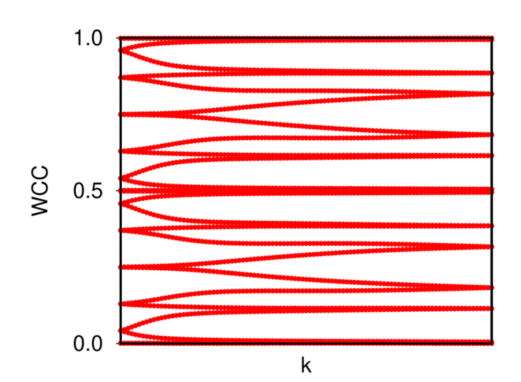
Wanniercenter_calc = T
/
&SYSTEM
NSLAB = 4 ! for thin film system
NSLAB1= 2 ! nanowire system
NSLAB2= 2 ! nanowire system
NumOccupied = 18 ! NumOccupied
SOC = 1 ! soc
E_FERMI = 4.4195 ! e-fermi, a global shift of the energy levels
surf_onsite= 0.0 ! surf_onsite
/
&PARAMETERS
Eta_Arc = 0.001 ! infinite small value, like brodening
E_arc = 0.0 ! energy level for contour plot of spectrum
OmegaNum = 400 ! omega number
OmegaMin = -0.6 ! energy interval
OmegaMax = 0.5 ! energy interval
Nk1 = 10 ! number k points odd number would be better
Nk2 = 10 ! number k points odd number would be better
Nk3 = 10 ! number k points odd number would be better
NP = 1 ! number of principle layers
Gap_threshold = 0.01 ! threshold for FindNodes_calc output
/
KPATH_BULK ! k point path
4 ! number of k line only for bulk band
G 0.00000 0.00000 0.0000 Z 0.00000 0.00000 0.5000
Z 0.00000 0.00000 0.5000 F 0.50000 0.50000 0.0000
F 0.50000 0.50000 0.0000 G 0.00000 0.00000 0.0000
G 0.00000 0.00000 0.0000 L 0.50000 0.00000 0.0000
KPATH_SLAB
2 ! numker of k line for 2D case
K 0.33 0.67 G 0.0 0.0 ! k path for 2D case
G 0.0 0.0 M 0.5 0.5
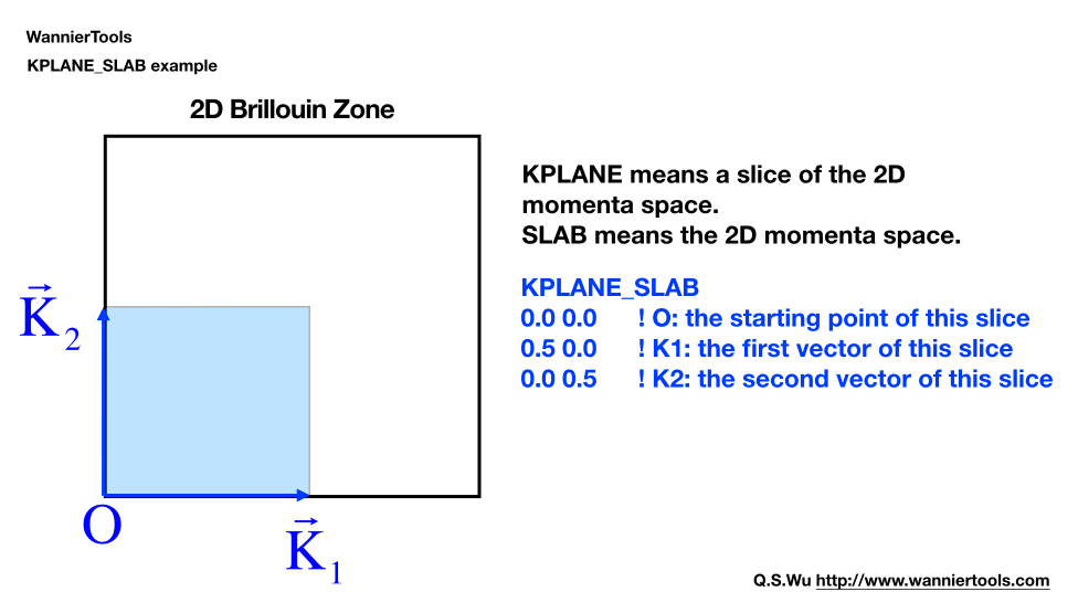
KPLANE_SLAB
-0.1 -0.1 ! Original point for 2D k plane
0.2 0.0 ! The first vector to define 2D k plane
0.0 0.2 ! The second vector to define 2D k plane for arc plots
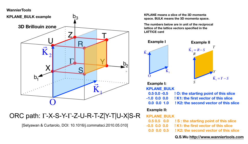
KPLANE_BULK
0.00 0.00 0.50 ! Original point for 3D k plane
1.00 0.00 0.00 ! The first vector to define 3d k space plane
0.00 0.50 0.00 ! The second vector to define 3d k space plane
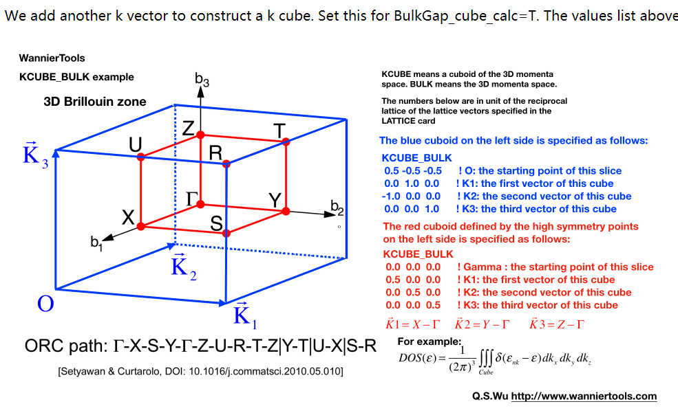
KCUBE_BULK
-0.50 -0.50 -0.50 ! Original point for 3D k plane
1.00 0.00 0.00 ! The first vector to define 3d k space plane
0.00 1.00 0.00 ! The second vector to define 3d k space plane
0.00 0.00 1.00 ! The third vector to define 3d k cube
WANNIER_CENTRES ! copy from wannier90.wout
Cartesian
-0.000040 -1.194745 6.638646
0.000038 -1.196699 6.640059
-0.000032 -1.192363 6.640243
-0.000086 -3.583414 2.908040
0.000047 -3.581457 2.906587
-0.000033 -3.585864 2.906443
-0.000001 1.194527 4.773338
0.000003 1.194538 4.773336
-0.000037 1.194536 4.773327
0.000006 -1.194384 1.130261
-0.000018 -1.216986 1.140267
0.000007 -1.172216 1.140684
0.000011 -3.583770 8.416406
-0.000002 -3.561169 8.406398
-0.000007 -3.605960 8.405979
0.000086 -1.194737 6.638626
-0.000047 -1.196693 6.640080
0.000033 -1.192286 6.640223
0.000040 -3.583406 2.908021
-0.000038 -3.581452 2.906608
0.000032 -3.585788 2.906424
0.000001 1.194548 4.773330
-0.000003 1.194537 4.773332
0.000037 1.194539 4.773340
-0.000011 -1.194381 1.130260
0.000002 -1.216981 1.140268
0.000007 -1.172191 1.140687
-0.000006 -3.583766 8.416405
0.000018 -3.561165 8.406400
-0.000007 -3.605935 8.405982
设置紧束缚哈密顿量
&TB_FILE  ! 输入控制文件中共有4个这样的名字 TB_FILE, SYSTEM, CONTROL, PARAMETERS,分别用来控制不同内容
Hrfile = 'wannier90_hr.dat'  ! 紧束缚哈密顿量的位置
Package = 'VASP'             ! obtained from VASP, it could be 'VASP', 'QE', 'Wien2k', 'OpenMx'
/
设置体系的一些性质
&SYSTEM
Nslab = 10  !Number of slabs for slab band, The default value is 10
Nslab1= 6   ! The thickness of nano ribbon
Nslab2= 6
NumOccupied = 18        ! 占据的Wannier能带的数目,这个设置一定要正确才行
SOC = 1                 ! SOC>0代表模型中考虑自旋轨道耦合,SOC=0则代表不考虑自旋轨道耦合
E_FERMI = 4.4195        ! real-valued, Fermi level for the given tight binding model
Bx= 0, By= 0, Bz= 0     ! Bx By Bz
surf_onsite= 0.0        ! real-valued, Additional onsite energy on the surface, you can set this to see how surface state changes
/
计算控制
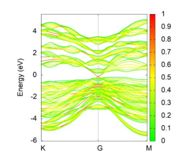
BulkBand_calc = T ! 计算体态能带
BulkFS_calc = F ! 体系费米面计算
BulkGap_cube_calc = F ! Energy gap for a given k cube for bulk system
BulkGap_plane_calc = F ! Energy gap for a given k plane for bulk system
SlabBand_calc = T ! Band structure for 2D slab system(开边界能带计算)
WireBand_calc = F ! Band structure for 1D ribbon system(若为3D体系,则表示开两个方向边界进行计算)
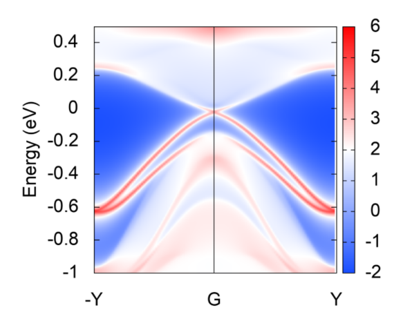
SlabSS_calc = T ! Surface spectrum A(k,E) along a kline and energy interval for slab system(计算开边界时候的表面态)
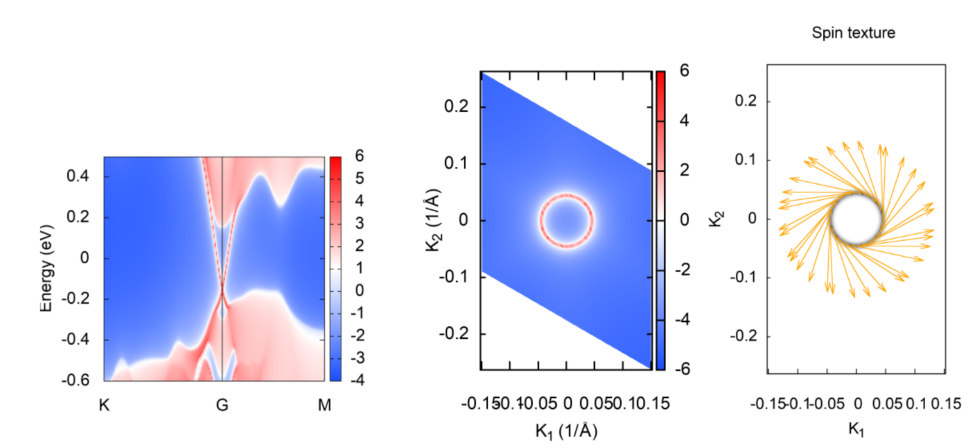
SlabArc_calc = F ! Surface spectrum A(k,E0) for fixed energy E0 in 2D k-plane for slab system (计算确定能量下的表面态)
SlabSpintexture_calc = T ! Spin texture in 2D k-plane for slab system(开边界表面态上的自旋分布计算)
wanniercenter_calc = F ! 计算Wannier Center的变化
BerryCurvature_calc = F ! 计算体系Berry曲率
/
参数设置
E_arc = 0.0         ! 计算费米弧时候的能量
Eta_Arc = 0.001     ! infinite small value, like broadening(格林函数的小虚部)
OmegaNum = 200      ! omega number
OmegaMin = -0.6     ! energy interval
OmegaMax =  0.5     ! energy interval
Nk1 = 50            ! number k points
Nk2 = 50            ! number k points
Nk3 = 50            ! number k points
NP = 2              ! You need to do a convergence test by setting Np= 1, Np=2, Np=3, and check the surface state spectrum.
                    !  Basically, the value of Np depends on the spread of Wannier functions you constructed. One thing should
                    ! be mentioned is that the computational time grows cubically of Np.
Gap_threshold = 1.0 !This value is used when you do energy gap calculation like BulkGap_cube_calc=T
/
晶体结构信息设置
LATTICE
Angstrom ! 长度单位
-2.069  -3.583614  0.000000     ! 元胞基矢
 2.069  -3.583614  0.000000
 0.000   2.389075  9.546667
原子位置
ATOM_POSITIONS
5                               ! 元胞内有5个原子
Direct                          ! 原子位置的表示方式
Bi 0.3990    0.3990    0.6970   ! 每个原子的位置坐标
Bi 0.6010    0.6010    0.3030
Se 0     0     0.5
Se 0.2060    0.2060    0.1180
Se 0.7940    0.7940    0.8820
轨道投影
PROJECTORS
 3 3 3 3 3          ! 每个原子的投影轨道数目
 Bi pz px py        ! 设置每个原子的投影轨道
 Bi pz px py
 Se pz px py
 Se pz px py
 Se pz px py
表面计算设置
SURFACE            ! 设置要研究的是哪个面上的性质
 1  0  0           ! a11, a12, a13
 0  1  0           ! a21 a22 a23
体态能带计算
KPATH_BULK            ! 计算体态能带时,动量空间中路径的选择
4              ! number of k line only for bulk band
G 0.00000 0.00000 0.0000 Z 0.00000 0.00000 0.5000
Z 0.00000 0.00000 0.5000 F 0.50000 0.50000 0.0000
F 0.50000 0.50000 0.0000 G 0.00000 0.00000 0.0000
G 0.00000 0.00000 0.0000 L 0.50000 0.00000 0.0000
特殊点能带计算
KPOINTS_3D  !You can calculate the properties on some kpoints you specified in point mode
4              ! number of k points
Direct         ! Direct or Cartesian
0.00000 0.00000 0.0000
0.00000 0.00000 0.5000
0.50000 0.50000 0.0000
0.00000 0.00000 0.0000
slab结构计算表面态
KPATH_SLAB  ! 计算表面态时候的路径选择
2        ! numker of k line for 2D case
K 0.33 0.67 G 0.0 0.0  ! k path for 2D case
G 0.0 0.0 M 0.5 0.5
2D平面上arc计算
KPLANE_SLAB
-0.1 -0.1      ! Original point for 2D k plane
 0.2  0.0      ! The first vector to define 2D k plane
 0.0  0.2      ! The second vector to define 2D k plane  for arc plots
3D体BZ中的计算
KPLANE_BULK
-0.50 -0.50  0.00   ! Original point for 3D k plane
 1.00  0.00  0.00   ! The first vector to define 3d k space plane
 0.00  1.00  0.00   ! The second vector to define 3d k space plane
KCUBE_BULK
KCUBE_BULK
-0.50 -0.50 -0.50   ! Original point for 3D k plane
 1.00  0.00  0.00   ! The first vector to define 3d k space plane
 0.00  1.00  0.00   ! The second vector to define 3d k space plane
 0.00  0.00  1.00   ! The third vector to define 3d k cube
Wannier Center计算
WANNIER_CENTRES     ! copy from wannier90.wout(需要结合Wannier90来产生数据)
Cartesian
 -0.000040  -1.194745   6.638646
  0.000038  -1.196699   6.640059
 -0.000032  -1.192363   6.640243
 -0.000086  -3.583414   2.908040
  0.000047  -3.581457   2.906587
 -0.000033  -3.585864   2.906443
 -0.000001   1.194527   4.773338
  0.000003   1.194538   4.773336
 -0.000037   1.194536   4.773327
  0.000006  -1.194384   1.130261
 -0.000018  -1.216986   1.140267
  0.000007  -1.172216   1.140684
  0.000011  -3.583770   8.416406
 -0.000002  -3.561169   8.406398
 -0.000007  -3.605960   8.405979
  0.000086  -1.194737   6.638626
 -0.000047  -1.196693   6.640080
  0.000033  -1.192286   6.640223
  0.000040  -3.583406   2.908021
 -0.000038  -3.581452   2.906608
  0.000032  -3.585788   2.906424
  0.000001   1.194548   4.773330
 -0.000003   1.194537   4.773332
  0.000037   1.194539   4.773340
 -0.000011  -1.194381   1.130260
  0.000002  -1.216981   1.140268
  0.000007  -1.172191   1.140687
 -0.000006  -3.583766   8.416405
  0.000018  -3.561165   8.406400
 -0.000007  -3.605935   8.405982
结果
公众号
相关内容均会在公众号进行同步,若对该Blog感兴趣,欢迎关注微信公众号。

|
yxli406@gmail.com |