借助Fortran格式化Julia输出的数据
在利用Julia做计算的时候,始终不能将数据整理成格式化的形式,这里就只好借助于Fortran来将其输出的数据重新读入之后,在进行格式化操作,最后再输出了.先以一个Julia计算的程序为例1
2
3
4
5
6
7
8
9
10
11
12
13
14
15
16
17
18
19
20
21
22
23
24
25
26
27
28
29
30
31
32
33
34
35
36
37
38
39
40
41
42
43
44
45
46
47
48
49
50
51
52
53
54
55
56
57
58
59
60
61
62
63
64
65
66
67
68
69
70
71
72
73
74
75
76
77
78
79
80
81
82
83
84
85
86
87
88
89
90
91
92
93
94
95
96
97
98
99
100
101
102
103
104
105
106
107
108
109
110
111
112
113
114
115
116
117
118
119
120
121
122
123
124
125
126
127
128
129
130
131
132using LinearAlgebra,DelimitedFiles,PyPlot
#---------------------------------------------------
function Pauli()
hn = 4
g1 = zeros(ComplexF64,hn,hn)
g2 = zeros(ComplexF64,hn,hn)
g3 = zeros(ComplexF64,hn,hn)
#------ Kinetic energy
g1[1,1] = 1
g1[2,2] = -1
g1[3,3] = 1
g1[4,4] = -1
#-------- SOC-x
g2[1,2] = 1
g2[2,1] = 1
g2[3,4] = -1
g2[4,3] = -1
#---------- SOC-y
g3[1,2] = -1im
g3[2,1] = 1im
g3[3,4] = -1im
g3[4,3] = 1im
return g1,g2,g3
end
# ========================================================
function matset(ky::Float64)
hn::Int64 = 4
H00 = zeros(ComplexF64,4,4)
H01 = zeros(ComplexF64,4,4)
g1 = zeros(ComplexF64,4,4)
g2 = zeros(ComplexF64,4,4)
g3 = zeros(ComplexF64,4,4)
#--------------------
m0::Float64 = 1.5
tx::Float64 = 1.0
ty::Float64 = 1.0
ax::Float64 = 1.0
ay::Float64 = 1.0
g1,g2,g3 = Pauli()
#--------------------
for m in 1:hn
for l in 1:hn
H00[m,l] = (m0-ty*cos(ky))*g1[m,l] + ay*sin(ky)*g3[m,l]
H01[m,l] = (-tx*g1[m,l] - 1im*ax*g2[m,l])/2
end
end
#------
return H00,H01
end
# ====================================================================================
function surfgreen_1985(omg::Float64,ky::Float64)
hn::Int64 = 4
GLL = zeros(ComplexF64,hn,hn)
GRR = zeros(ComplexF64,hn,hn)
GBulk = zeros(ComplexF64,hn,hn)
iter::Int64 = 0
itermax::Int64 = 100
accuarrcy::Float64 = 1E-7
real_temp::Float64 = 0.0
omegac::ComplexF64 = 0.0
eta::Float64 = 0.01
#-----------------------------------
alphai = zeros(ComplexF64,hn,hn)
betai = zeros(ComplexF64,hn,hn)
epsiloni = zeros(ComplexF64,hn,hn)
epsilons = zeros(ComplexF64,hn,hn)
epsilons_t = zeros(ComplexF64,hn,hn)
mat1 = zeros(ComplexF64,hn,hn)
mat2 = zeros(ComplexF64,hn,hn)
g0 = zeros(ComplexF64,hn,hn)
unit = zeros(ComplexF64,hn,hn)
#------------------------------------
H00,H01 = matset(ky)
epsiloni = H00
epsilons = H00
epsilons_t = H00
alphai = H01
betai = conj(transpose(H01))
#-------------------------------------
for i in 1:hn
unit[i,i] = 1
end
#-------------------------------------
omegac = omg + 1im*eta
for iter in 1:itermax
g0 = inv(omegac*unit- epsiloni)
mat1 = alphai*g0
mat2 = betai*g0
g0 = mat1*betai
epsiloni = epsiloni + g0
epsilons = epsilons + g0
g0 = mat2*alphai
epsiloni= epsiloni + g0
epsilons_t = epsilons_t+ g0
g0 = mat1*alphai
alphai = g0
betai = g0
real_temp = abs(sum(alphai))
if real_temp < accuarrcy
break
end
end
GLL = inv(omegac*unit - epsilons)
GRR = inv(omegac*unit - epsilons_t)
GBulk = inv(omegac*unit - epsiloni)
return GLL,GRR,GBulk
end
# ==========================================================
function surfState()
hn::Int64 = 4
dk::Float64 = 0.01
domg::Float64 = 0.01
ky::Float64 = 0.0
omg::Float64 = 0.0
GLL = zeros(ComplexF64,hn,hn)
GRR = zeros(ComplexF64,hn,hn)
GBulk = zeros(ComplexF64,hn,hn)
f1 = open("edgeState.dat","w")
for ky in -pi:dk:pi
for omg in -3:domg:3
GLL,GRR,GBulk = surfgreen_1985(omg,ky)
re1 = -imag(sum(GLL))/pi
re2 = -imag(sum(GRR))/pi
re3 = -imag(sum(GBulk))/pi
writedlm(f1,[ky/pi omg re1 re2 re3])
end
end
close(f1)
end
# =========================================================
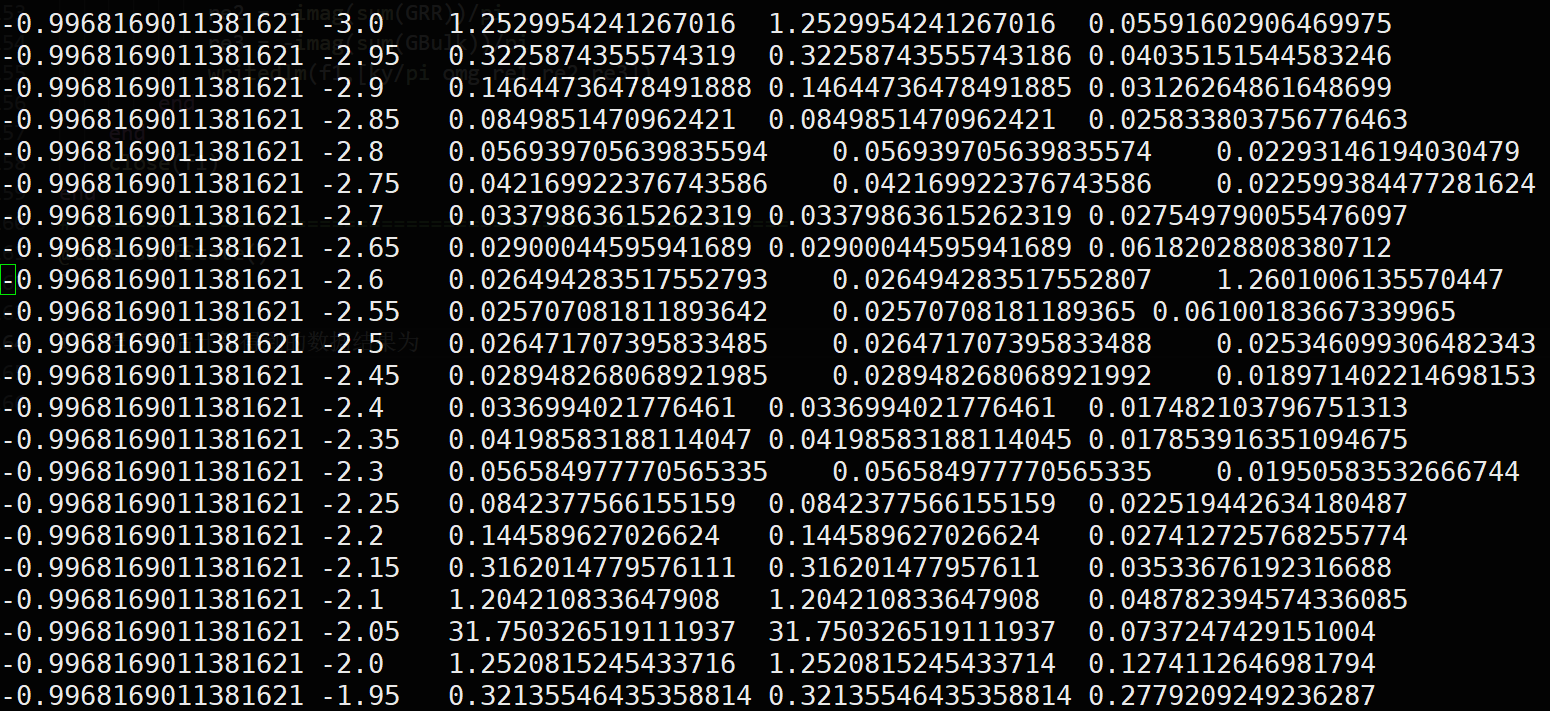
surfState()
这个程序最后计算得到的数据结果为
可以发现这样的数据格式非常不整齐,不太利于之后的操作,所以接下来就通过Fortran程序将这个数据文件读入,然后再格式化输出.1
2
3
4
5
6
7
8
9
10
11
12
13
14
15
16
17
18
19
20
21
22
23
24
25
26
27
28
29
30
31
32
33
34 program main
implicit none
integer m1,m2,m3
call main1()
stop
end program
!=======================================================
subroutine main1()
! 读取不明行数的文件
implicit none
integer count,stat
real h1,h2,h3,h4,h5,h22
h1 = 0
h2 = 0
h3 = 0
h22 = 0
open(1,file = "test.dat")
open(2,file = "test-format.dat")
count = 0
do while (.true.)
     count = count + 1
     h22 = h1
     read(1,*,iostat = STAT)h1,h2,h3,h4,h5
     if(h22.ne.h1)write(2,*)""  ! 在这里加空行是为了gnuplot绘制密度图
     write(2,999)h1,h2,h3,h4,h5   ! 数据格式化
     if(stat .ne. 0) exit ! 当这个参数不为零的时候,证明读取到文件结尾
 end do
! write(*,*)h1,h2,h3
! write(*,*)count
close(1)
close(2)
999 format(10f11.6)
return
end subroutine main1
首先来解释一下程序中的内容,因为再计算的时候,数据第一列是外部循环变量,所以先取定一个值保持不变,第二列的值遍历一次循环.因此当1
2
3
4
5
6
7
8do while (.true.)
count = count + 1
h22 = h1
read(1,*,iostat = STAT)h1,h2,h3,h4,h5
if(h22.ne.h1)write(2,*)"" ! 在这里加空行是为了gnuplot绘制密度图
write(2,999)h1,h2,h3,h4,h5 ! 数据格式化
if(stat .ne. 0) exit ! 当这个参数不为零的时候,证明读取到文件结尾
end do
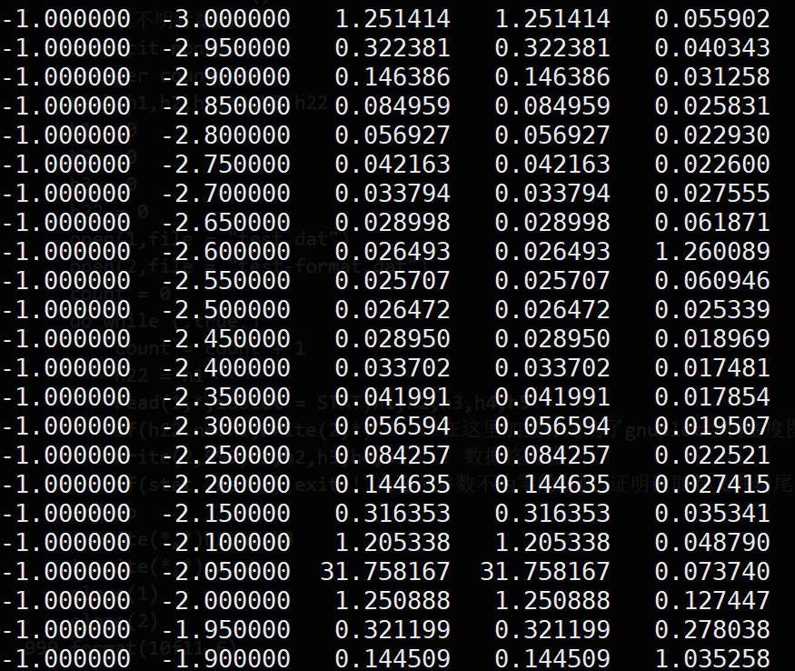
第一列的值在读取的时候,不相等了,说明开始读取下一次外层循环了,这里就多加了一行空格,是为了利用gnuplot绘制密度图所用.而在文件读取的时候1
read(1,*,iostat = STAT)h1,h2,h3,h4,h5
STAT这个量会反应是否读取到了文件的末尾,从而来判断循环过程时候中断.最后得到的数据如下图所示
将数据整理格式化之后,就可以利用gnuplot来绘制图像了1
2
3
4
5
6
7
8
9
10
11
12
13
14
15
16
17
18
19
20
21
22
23
24
25
26
27
28
29set encoding iso_8859_1
set terminal postscript enhanced color
set output 'arc_r.eps'
set terminal pngcairo truecolor enhanced font ",50" size 1920, 1680
set terminal png truecolor enhanced font ",50" size 1920, 1680
set output 'density.png'
set palette defined ( -10 "#194eff", 0 "white", 10 "red" )
set palette defined ( -10 "blue", 0 "white", 10 "red" )
set palette rgbformulae 33,13,10
unset ztics
unset key
set pm3d
set border lw 6
set size ratio 1
set view map
set xtics
set ytics
set xlabel "K_1 (1/{\305})"
set xlabel "X_1"
set ylabel "K_2 (1/{\305})"
set ylabel "Y"
set ylabel offset 1, 0
set colorbox
set xrange [-1:1]
set yrange [-3:3]
set pm3d interpolate 4,4
splot 'wavenorm.dat' u 1:2:3 w pm3d
splot 'wavenorm.dat' u 1:2:3 w pm3d
splot 'test-format.dat' u 1:2:3 w pm3d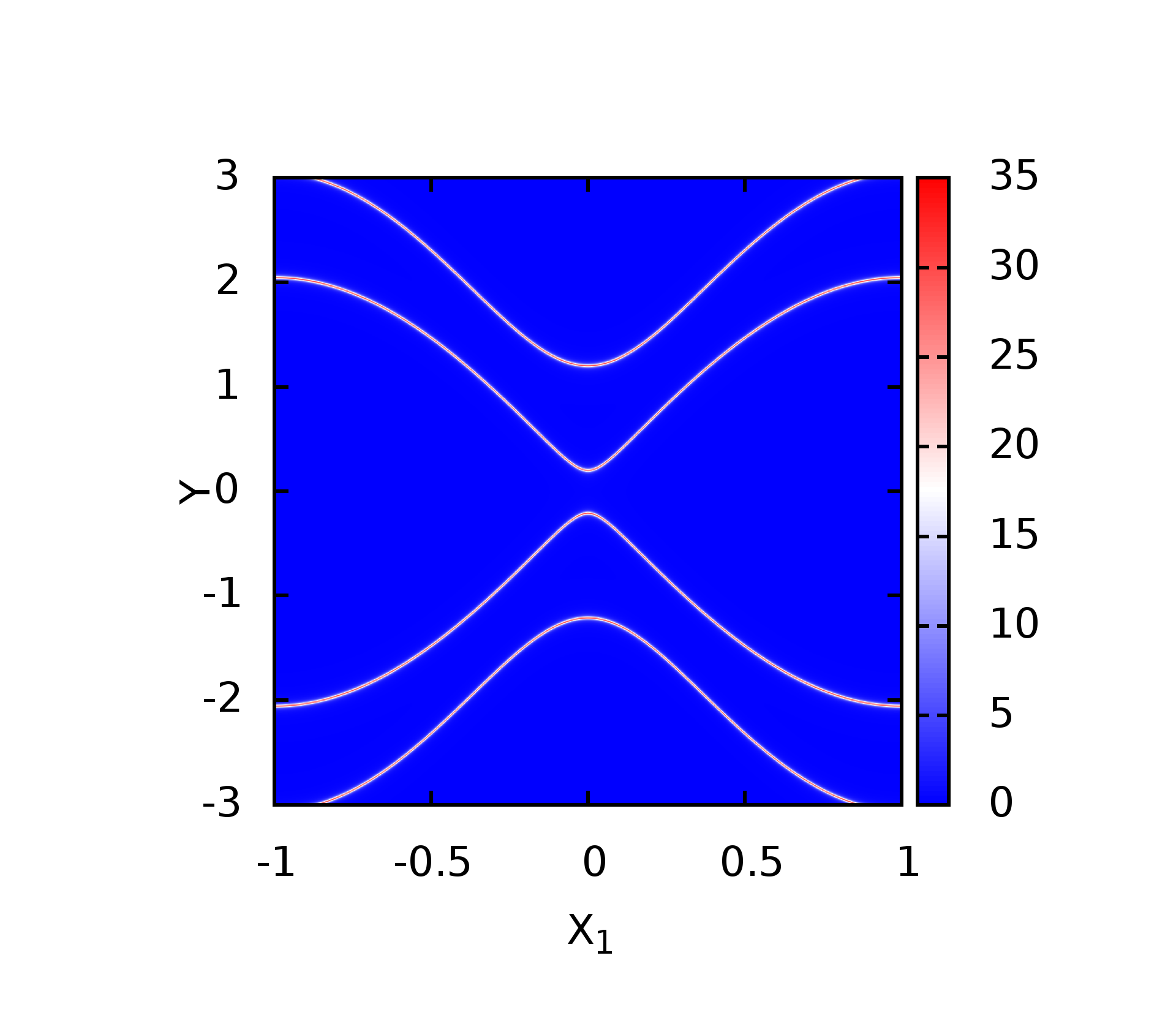
因为利用格林函数方法进行计算的时候,要想得到漂亮的图,取点间隔必须小,这样就会使得数据比较大,所以利用gnuplot绘图还是比较方便的.
代码下载
这些程序的源代码,可以点击这里下载
鉴于该网站分享的大都是学习笔记,作者水平有限,若发现有问题可以发邮件给我
- yxliphy@gmail.com
也非常欢迎喜欢分享的小伙伴投稿


欢迎关注公众号,有趣的内容也会在上面同步。 有密码的文章属于正在建设中或者没有通过验证的内容,若有需要可通过邮件联系。