BHZ模型Wilson loop计算
这里整理一下计算BHZ模型Wilson loop的代码.
{:.info}
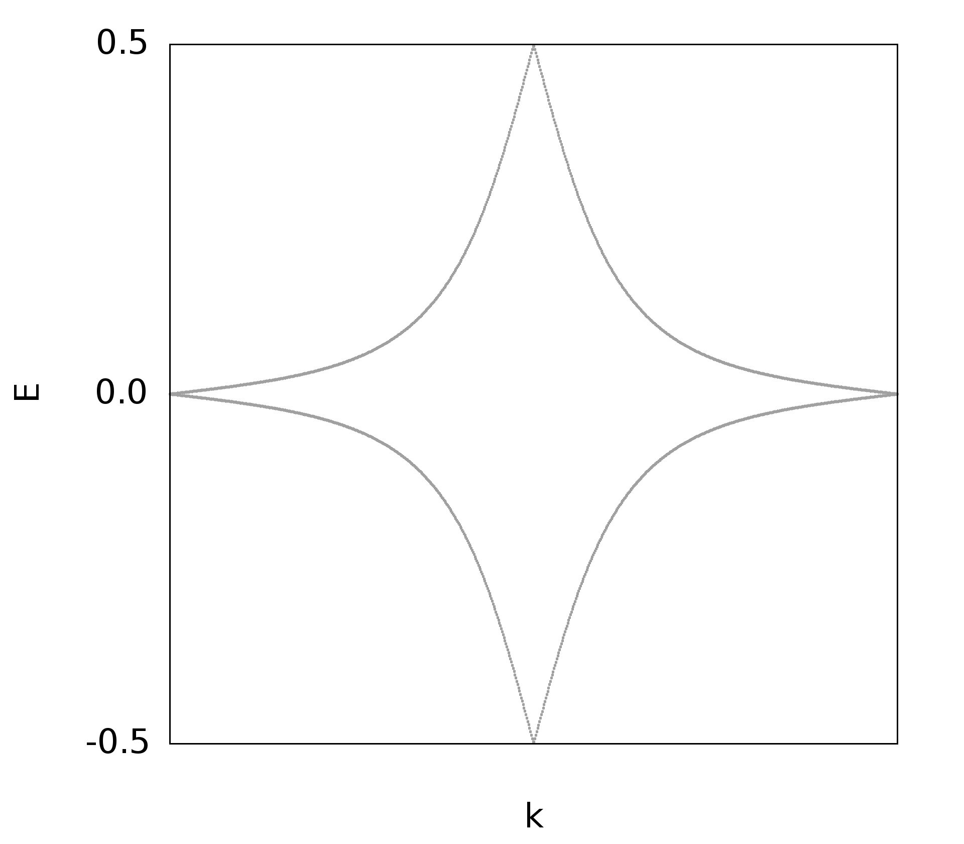
BHZ模型是最初学习拓扑时接触比较早的模型,前面也整理过如何计算BHZ模型的$\mathcal{Z}_2$拓扑不变量,但是其拓扑性质仍然可以通过Wilson loop来进行计算,所以这里就利用Julia来计算一下这个模型的Wilson loop.
代码
1 | using LinearAlgebra,PyPlot,DelimitedFiles |
- 计算结束后,利用`fortran``来将数据进行格式化
1
2
3
4
5
6
7
8
9
10
11
12
13
14
15
16
17
18
19
20
21
22
23
24
25
26
27
28
29
30
31
32
33
34
35
36
program main
implicit none
integer m1,m2,m3
call main1()
stop
end program
!=======================================================
subroutine main1()
! 读取不明行数的文件
implicit none
integer count,stat
real h1,h2,h3,h4,h5,h22
h1 = 0
h2 = 0
h3 = 0
h22 = 0
open(1,file = "test.dat")
open(2,file = "test-format.dat")
count = 0
do while (.true.)
count = count + 1
h22 = h1
! read(1,*,iostat = STAT)h1,h2,h3,h4,h5
read(1,*,iostat = STAT)h1,h2,h3
! if(h22.ne.h1)write(2,*)"" ! 在这里加空行是为了gnuplot绘制密度图
! write(2,999)h1,h2,h3,h4,h5 ! 数据格式化
write(2,999)h1,h2,h3 ! 数据格式化
if(stat .ne. 0) exit ! 当这个参数不为零的时候,证明读取到文件结尾
end do
! write(*,*)h1,h2,h3
! write(*,*)count
close(1)
close(2)
999 format(5f11.6)
return
end subroutine main1
绘图
1 | set encoding iso_8859_1 |
参考
公众号
相关内容均会在公众号进行同步,若对该Blog感兴趣,欢迎关注微信公众号。
{:.info}

|
yxliphy@gmail.com |
本博客所有文章除特别声明外,均采用 CC BY-NC-SA 4.0 许可协议。转载请注明来源 Yu-Xuan's Blog!
 wechat
 alipay
相关推荐
2019-04-17
Majorana Corner State in High Temperature Superconductor
最近刚刚学习了julia, 手头上也正好在重复一篇文章,就正好拿新学习的内容一边温习一边做研究。{:.success} 导入函数库1234567# Import external package that used in program import Pkg# Pkg.add("PyPlot")# Pkg.add("LinearAlgebra")# Pkg.add("CPUTime")...
2020-07-01
两种方法计算Chern Number
计算Chern数是最初学习拓扑物理都会遇到的问题,正好在假期空闲的时候自己学习了一下Chern数的数值计算方法,在博客上记录一下希望可以帮助到别人。{:.info}具体的计算方法和细节就不在这里说明了,只要是想学习计算Chern数的肯定了解它在凝聚态物理中的角色,而计算的细节也会在后面的参考文献中给出,只是展示一下结果。 Julia语言计算Chern numberVersion1这个方法是直接用定义直接计算的结果,但是可能会遇到波函数规范选择的问题,会导致结果有误,而具体的规范问题,我并不懂,所以一般我会选择第二种方法来计算,也就是后面参考文献中介绍的方法。1234567891011121314151617181920212223242526272829303132333435363738394041424344454647484950515253545556575859606162636465666768697071727374import PkgPkg.add("LinearAlgebra")Pkg.add("PyPlot")using LinearAlgebra,PyPlotfunction matSet(kx::Float64,ky::Float64)::Matrix{ComplexF64} m0::Float64 = -1.0 t1::Float64 = 1.0 t2::Float64 = 1.0 t3::Float64 = 0.5 # 这里选取的是量子反常Hall效应的模型 ham = zeros(ComplexF64,2,2) ham[1,1] = m0 + 2*t3*sin(kx) + 2*t3*sin(ky) + 2*t2*cos(kx + ky) ham[2,2] = -(m0 + 2*t3*sin(kx) + 2*t3*sin(ky) + 2*t2*cos(kx + ky)) ham[1,2] = 2*t1*cos(kx) - 1im*2*t1*cos(ky) ham[2,1] = conj(ham[1,2]) return...
2020-06-30
Kane Mele model zigzag 边界态的计算
接触量子自旋霍尔效应很久了,但是一直也都是在square lattice上做计算,从来没有认真的在六角点阵上计算过拓扑的内容,正好最近在看文献的过程中需要在石墨烯机构上进行,就从最基本的Kane-Mele 模型出发学习怎么在六角点阵上写出最近邻以及次近邻的哈密顿量。{:.info}关于最近邻之间的hopping在前面石墨烯的边界态文章中已经仔细考虑过,包括cell的选取还有原子的编号,在这里。现在唯一的不同就是要考虑次近邻之间的hopping。在这里暂时并未考虑Rashbo自旋轨道耦合。 基本设定 蓝色虚线框中是选择的一个大cell,在y方向是有限长度,在x方向是无限的,所以$k_x$是个好量子数,这种边界态叫zigzag;当x方向开边界,y方向无限长时的边界态叫armchair,可以参考这里。格点之间的hopping可以在一个大cell之内,可会存在大cell之间的hopping,在下面会逐一展示。关于Kane-Mele模型中的$v_{ij}$的示意如上图_hopping_蓝色箭头所示,当格点连线在hopping的右侧时$v_{ij}=-1$,在左侧时$v_{ij}=1$;将一个大cell划分成更小的周期重复结构,如上图右下图所示,并分别编号。第一张图所示的是最近邻hopping的选择。 H = t_1\sum_{\alpha}c_{i\alpha}^\dagger c_{j\alpha})+it_2\sum_{\alpha\beta}v_{i,j}s^z_{\alpha\beta}c_{i\alpha}^\dagger c_{j\beta}与之前的Graphene模型相比较,这里是有两个自旋的,不过唯一的影响的只是第二项,对于上下自旋的不同相差一个符号,并不会对hopping的分析有影响。 次近邻hopping 在虚线框中的是一个大cell,在右侧的是一个小cell,在写Hamiltonian的时候是以小cell为基本单元进行的。 首先可以看到,无论是边界上的小cell还是非边界上的小cell,都会具有如图中紫色虚线箭头所示的次近邻hopping,而且这些hopping是在同一个大cell内的。这种情况中格点连线都在hopping线的右端$v_{ij} =...
评论