之前其实已经研究过BBH模型的拓扑性质,但是一直没去写实空间电荷分布以及零能态的代码,这里补一下作业。
模型
废话不说,直接给模型上代码,具体的性质可以参考Electric multipole moments, topological multipole moment pumping, and chiral hinge states in crystalline insulators这篇文章。
\[\begin{aligned} h^{q}(\mathbf{k})=& {\left[\gamma_{x}+\lambda_{x} \cos \left(k_{x}\right)\right] \Gamma_{4}+\lambda_{x} \sin \left(k_{x}\right) \Gamma_{3} } \\ &+\left[\gamma_{y}+\lambda_{y} \cos \left(k_{y}\right)\right] \Gamma_{2}+\lambda_{y} \sin \left(k_{y}\right) \Gamma_{1} \end{aligned}\]代码
using ProgressMeter
@everywhere using SharedArrays, LinearAlgebra,Distributed,DelimitedFiles,Printf
# --------------------------------------
@everywhere function boundary(xn::Int64,yn::Int64)
    len2::Int64 = xn*yn
    bry = zeros(Int64,4,len2)
    for iy in 1:yn
        for ix in 1:xn
            i = (iy - 1)*xn + ix
            bry[1,i] = i + 1
            if ix == xn
                bry[1,i] = bry[1,i] - xn
            end
            bry[2,i] = i - 1
            if ix == 1
                bry[2,i] = bry[2,i] + xn
            end
            bry[3,i] = i + xn
            if iy == yn
                bry[3,i] = bry[3,i] - len2
            end
            bry[4,i] = i - xn
            if iy == 1
                bry[4,i] = bry[4,i] + len2
            end
        end
    end
    return bry
end
#-------------------------------------
@everywhere function pauli()
    s0 = zeros(ComplexF64,2,2)
    s1 = zeros(ComplexF64,2,2)
    s2 = zeros(ComplexF64,2,2)
    s3 = zeros(ComplexF64,2,2)
    #----
    s0[1,1] = 1
    s0[2,2] = 1
    #----
    s1[1,2] = 1
    s1[2,1] = 1
    #----
    s2[1,2] = -im
    s2[2,1] = im
    #-----
    s3[1,1] = 1
    s3[2,2] = -1
    #-----
    return s0,s1,s2,s3
end
#---------------------------------------
@everywhere function gamma()
    s0,sx,sy,sz = pauli()
    g1 = -kron(sy,sx)
    g2 = -kron(sy,sy)
    g3 = -kron(sy,sz)
    g4 = kron(sx,s0)
    g5 = kron(sz,s0) # 微扰
    return g1,g2,g3,g4,g5
end
#---------------------------------------
@everywhere function matset(xn::Int64,yn::Int64)
    gamx::Float64 = 0.001
    gamy::Float64 = 0.001
    lamx::Float64 = 1.0
    lamy::Float64 = 1.0
    d0::Float64 = 0.001
    hn::Int64 = 4
    N::Int64 = xn*yn*hn
    len2::Int64 = xn*yn
    ham = zeros(ComplexF64,N,N)
    g1,g2,g3,g4,g5 = gamma()
    bry = boundary(xn,yn)
    #---
    for iy in 1:yn
        for ix in 1:xn
            i0 = (iy - 1)*xn + ix
            for i1 in 0:hn -1
                for i2 in 0:hn - 1
                    ham[i0 + len2*i1,i0 + len2*i2] = gamx*g4[i1 + 1,i2 + 1] + gamy*g2[i1 + 1,i2 + 1] + d0*g5[i1 + 1,i2 + 1]
                    if ix != xn
                        ham[i0 + len2*i1,bry[1,i0] + len2*i2] = lamx/2.0*g4[i1 + 1,i2 + 1] + lamx/(2*im)*g3[i1 + 1,i2 + 1]
                    end
                    if ix != 1
                        ham[i0 + len2*i1,bry[2,i0] + len2*i2] = lamx/2.0*g4[i1 + 1,i2 + 1] - lamx/(2*im)*g3[i1 + 1,i2 + 1]
                    end
                    if iy != yn
                        ham[i0 + len2*i1,bry[3,i0] + len2*i2] = lamy/2.0*g2[i1 + 1,i2 + 1] + lamy/(2*im)*g1[i1 + 1,i2 + 1]
                    end
                    if iy != 1
                        ham[i0 + len2*i1,bry[4,i0] + len2*i2] = lamy/2.0*g2[i1 + 1,i2 + 1] - lamy/(2*im)*g1[i1 + 1,i2 + 1]
                    end
                end
            end
        end
    end
    #-----------------------------------------
    if ishermitian(ham)
        val,vec = eigen(ham)
    else
        println("Hamiltonian is not hermitian")
        # break
    end
    # fx1 = "juliaval-" * string(h0) * ".dat"
    fx1 = "eigval.dat"
    f1 = open(fx1,"w")
    ind = (a->(@sprintf "%5.2f" a)).(range(1,length(val),length = length(val)))
    val2 = (a->(@sprintf "%15.8f" a)).(map(real,val))
    # writedlm(f1,map(real,val),"\t")
    writedlm(f1,[ind val2],"\t")
    close(f1)
    return map(real,val),vec
end
#----------------------------------------
@everywhere function delta(x::Float64)
    gamma::Float64 = 0.01
    return 1.0/pi*gamma/(x*x + gamma*gamma)
end
#----------------------------------------
@everywhere function ldos()
    xn::Int64 = 30
    yn::Int64 = xn
    hn::Int64 = 4
    len2::Int64 = xn*yn
    N::Int64 = xn*yn*hn
    omg::Float64 = 0.0
    val,vec = matset(xn,yn)
    # fx1 = "juldos-" * string(h0) * ".dat"
    fx1 = "dos.dat"
    f1 = open(fx1,"w")
    for iy in 1:yn
        for ix in 1:xn
            i0 = (iy - 1)*xn + ix
            re1 = 0
            re2 = 0
            for ie in 1:N
                for i1 in 0:hn - 1
                    re1 = re1 + delta(val[ie] - omg)*(abs(vec[i0 + len2*i1,ie])^2)
                end
            end
            for ie in 1:Int(N/2)
                for i1 in 0:hn - 1
                    re2 += abs(vec[i0 + len2*i1,ie])^2
                end
            end
            @printf(f1,"%5.2f\t%5.2f\t%15.8f\t%15.8f\n",ix,iy,re1,re2)
            # writedlm(f1,[ix iy re1 re2],"\t")
        end
    end
    close(f1)
end
#--------------------------------------
# main()
@time ldos()
绘图
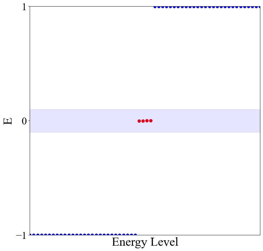
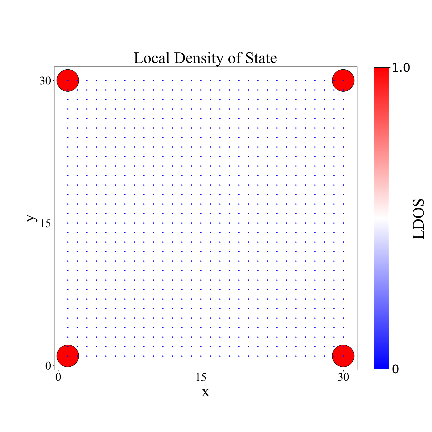
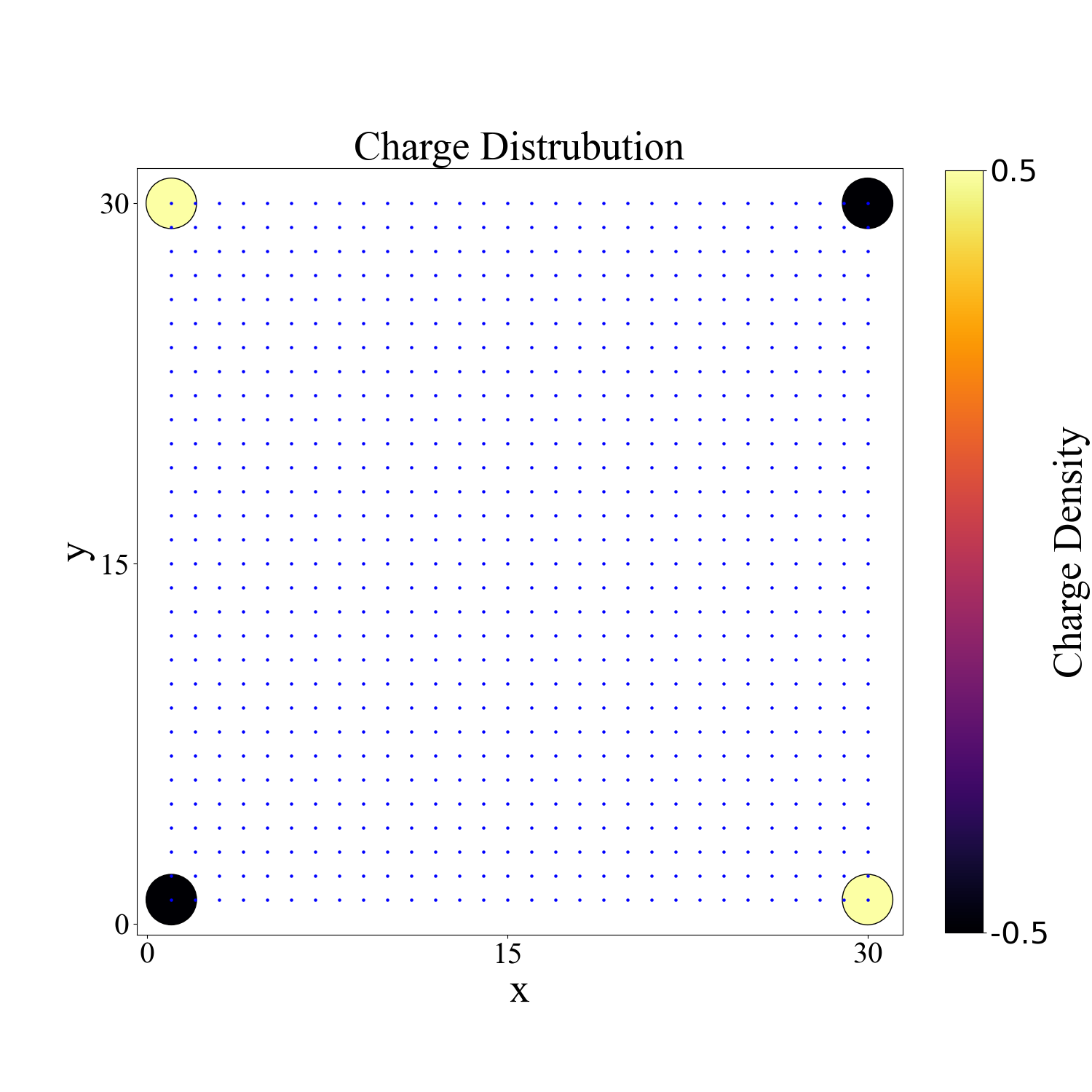
Julia目前画图调整方面我不是很熟悉,所以暂时先用Python作图了。分别给出实空间的本征值,态密度,残余电荷
import numpy as np
import matplotlib.pyplot as plt
import os

#---------------------------------------------------------
def ldosplt(cont):
    dataname = "m1-ldos-" + str(cont).rjust(2,'0') + ".dat"
    dataname = "dos.dat"
    picname = "ldos-m1-" + str(cont).rjust(2,'0') + ".png"
    os.chdir(os.getcwd())# 确定用户执行路径
    x0 = []
    y0 = []
    z0 = []
    z1 = []
    with open(dataname) as file:
        da = file.readlines()
        for f1 in da:
            if len(f1) > 3:
                ldos = [float(x) for x in f1.strip().split()]
                x0.append(ldos[0])
                y0.append(ldos[1])
                z0.append(ldos[2])
                z1.append(ldos[3])
    z0 = (z0 - np.min(z0))/(np.max(z0) - np.min(z0))*3000 # 数据归一化
    plt.figure(figsize=(15, 15))
    sc = plt.scatter(x0, y0, c = z0,s = z0,vmin=0, vmax=1,cmap="bwr",edgecolor="black")
    cb = plt.colorbar(sc,fraction = 0.045)  # 调整colorbar的大小和图之间的间距
    cb.ax.tick_params(labelsize = 30)
    cb.set_ticks(np.linspace(0,1,2))
    cb.set_ticklabels(('0','1.0'))

    font2 = {'family': 'Times New Roman',
             'weight': 'normal',
             'size': 40,
             }
    cb.set_label('LDOS',fontdict=font2) #设置colorbar的标签字体及其大小
    plt.scatter(x0, y0, s = 5, color='blue',edgecolor="blue")
    plt.axis('scaled')
    plt.xlabel("x",font2)
    plt.ylabel("y",font2)
    plt.title("Local Density of State",font2)
    plt.yticks([0,15,30],fontproperties='Times New Roman', size = 30)
    plt.xticks([0,15,30],fontproperties='Times New Roman', size = 30)
    plt.savefig(picname, dpi = 100)
    plt.close()
#---------------------------------------------------------
def eigval(cont):
    dataname = "eigval-m1-" + str(cont).rjust(4,'0') + ".dat"
    dataname = "eigval.dat"
    picname = "m1-val-" + str(cont).rjust(4,'0') + ".png"
    x0 = []
    y0 = []
    with open(dataname) as file:
        da = file.readlines()
        for f1 in da:
            if len(f1) > 2:
                da1 = [float(x) for x in f1.strip().split()]
                x0.append(da1[0])
                y0.append(da1[1])
    # plt.plot(x0, y0)
    # plt.title("|C| = 1",size = 20,fontproperties='Times New Roman')
    datalen = int(len(x0)/2)
    vallen = 30
    len1 = int(len(y0)/2)
    y0 = y0[len1 - vallen:len1 + vallen]
    valmin = np.min(y0)
    valmax = np.max(y0)
    x0 = range(len(y0))
    #----------------------------------
    plt.figure(figsize=(10, 10))
    sc = plt.scatter(x0, y0, s = 40,c='blue')
    sc = plt.scatter(x0[int(len(x0)/2)-2:int(len(x0)/2)+2], y0[int(len(y0)/2)-2:int(len(y0)/2)+2], s = 50, c='red')
    #cb = plt.colorbar(sc,fraction=0.045)  # 调整colorbar的大小和图之间的间距
    #cb.ax.tick_params(labelsize=20)
    #plt.xlim(datalen - vallen,datalen + vallen)
    plt.xlim(np.min(x0),np.max(x0))
    plt.ylim(valmin, valmax)
    yrange = 0.1
    c1 = -yrange*np.ones(len(x0))
    c2 = yrange*np.ones(len(x0))
    plt.fill_between(x0, c1, c2, color = 'blue', alpha = 0.1)
    font2 = {'family': 'Times New Roman',
             'weight': 'normal',
             'size': 30,
             }
    plt.yticks(fontproperties='Times New Roman', size = 25)
    plt.ylabel("E", font2)
    plt.xlabel("Energy Level", font2)
    plt.xticks([])
    plt.yticks([-1,0,1])
    plt.savefig(picname, dpi = 100, bbox_inches = 'tight')
    plt.close()
#---------------------------------------------------------
def charge(cont):
    dataname = "ldos-" + str(cont).rjust(2,'0') + ".dat"
    dataname = "dos.dat"
    picname = "charge-" + str(cont).rjust(2,'0') + ".png"
    os.chdir(os.getcwd())# 确定用户执行路径
    x0 = []
    y0 = []
    z0 = []
    z1 = []
    with open(dataname) as file:
        da = file.readlines()
        for f1 in da:
            if len(f1) > 3:
                ldos = [float(x) for x in f1.strip().split()]
                x0.append(ldos[0])
                y0.append(ldos[1])
                z0.append(ldos[2])
                z1.append(ldos[3])
    z0 = (z0 - np.min(z0))/(np.max(z0) - np.min(z0))*500 # 数据归一化
    z2 = [abs(x-2)*5000 for x in z1] # 定义scatter的大小
    z3 = [(x-2)*1000 for x in z1] # 定义scatter的颜色,因为这里电荷有正有负
    plt.figure(figsize=(15, 15))
    # sc = plt.scatter(x0, y0, c = z0,s = z0,vmin=0, vmax=1,cmap="seismic",edgecolor="black")
    sc = plt.scatter(x0, y0, c = z3,s = z2,vmin=-0.5, vmax=0.5,cmap="inferno",edgecolor="black")  # 残余电荷密度
    cb = plt.colorbar(sc,fraction = 0.045)  # 调整colorbar的大小和图之间的间距
    cb.ax.tick_params(labelsize = 30)
    cb.set_ticks(np.linspace(-0.5,0.5,2))
    cb.set_ticklabels(('-0.5','0.5'))

    font2 = {'family': 'Times New Roman',
             'weight': 'normal',
             'size': 40,
             }
    cb.set_label('Charge Density',fontdict=font2) #设置colorbar的标签字体及其大小
    plt.scatter(x0, y0, s = 5, color='blue',edgecolor="blue")
    plt.axis('scaled')
    plt.xlabel("x",font2)
    plt.ylabel("y",font2)
    plt.title("Charge Distrubution",font2)
    plt.yticks([0,15,30],fontproperties='Times New Roman', size = 30)
    plt.xticks([0,15,30],fontproperties='Times New Roman', size = 30)
    plt.savefig(picname, dpi = 100)
    plt.close()

#---------------------------------------------------------
def main1():
    for i0 in range(1,2):
        ldosplt(i0)
        eigval(i0)
        charge(i0)
#---------------------------------------------------------
if __name__=="__main__":
    main1()
公众号
相关内容均会在公众号进行同步,若对该Blog感兴趣,欢迎关注微信公众号。

|
yxli406@gmail.com |