Julia并行计算cylinder边界态
模型
还是用我最熟悉的模型BHZ+Superconductor
具体怎么实现可以查阅我其他的博客,我这里直接就上代码了
代码
1 | using SharedArrays, LinearAlgebra,Distributed,DelimitedFiles,Printf |
绘图
Julia画图功能暂时不是很完善,所以就用Python来绘图了,下面上绘图代码1
2
3
4
5
6
7
8
9
10
11
12
13
14
15
16
17
18
19
20
21
22
23
24
25
26
27
28
29
30
31
32
33
34
35
36
37
38
39
40
41
42
43
44
45
46
47
48
49
50
51
52
53
54
55
56
57
58
59
60
61
62
63
64
65
66
67
68
69
70
71
72
73
74
75
76
77
78
79
80
81
82
83
84
85
86
87
88
89
90
91
92
93
94
95
96
97
98
99import numpy as np
import matplotlib.pyplot as plt
from matplotlib import rcParams
import os
config = {
"font.size": 30,
"mathtext.fontset":'stix',
"font.serif": ['SimSun'],
}
rcParams.update(config) # Latex 字体设置
#---------------------------------------------------------
def scatterplot1(cont):
#da1 = "m" + str(cont) + "-pro-ox" + ".dat"
#da2 = "m" + str(cont) + "-pro-oy" + ".dat"
#da1 = "ox-" + str(cont).rjust(2,'0') + ".dat"
da1 = "ox-" + str(cont) + ".dat"
picname = "ox-" + str(cont) + ".png"
os.chdir(os.getcwd())# 确定用户执行路径
x0 = []
y0 = []
with open(da1) as file:
da = file.readlines()
for f1 in da:
if len(f1) > 3:
ldos = [float(x) for x in f1.strip().split()]
x0.append(ldos)
#y0.append(ldos)
x0 = np.array(x0)
plt.figure(figsize=(8,8))
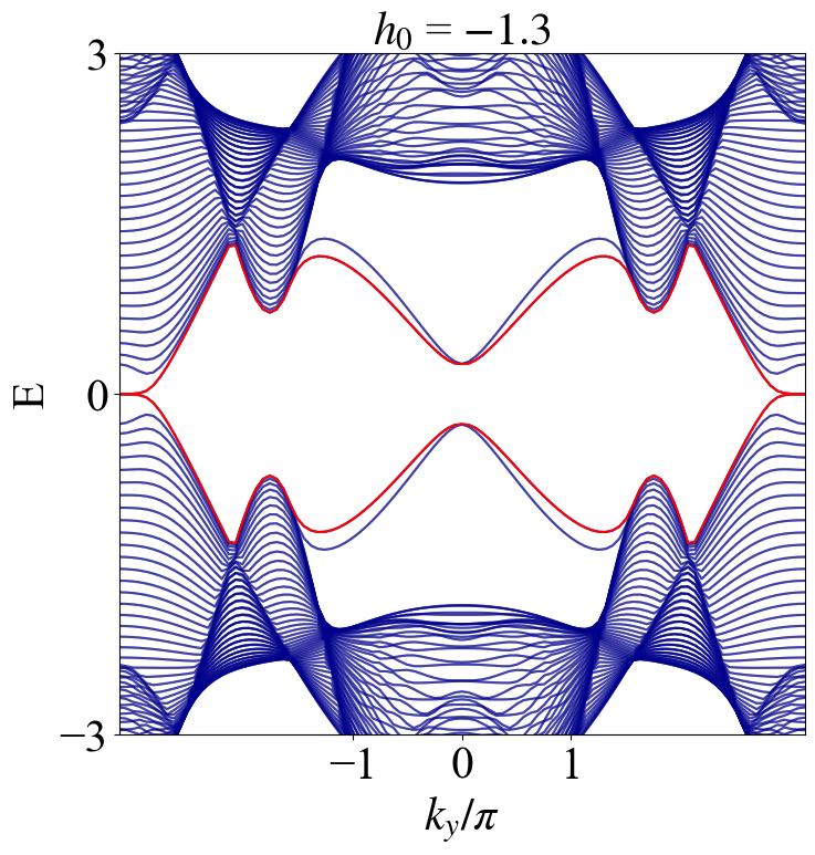
plt.plot(x0[:,0], x0[:,1:-1], c = 'darkblue', alpha = 0.5)
plt.plot(x0[:,0], x0[:,int(len(x0[1,:])/2)], c = 'red')
plt.plot(x0[:,0], x0[:,int(len(x0[1,:])/2) + 1], c = 'red')
x0min = np.min(x0[:,0])
x0max = np.max(x0[:,0])
font2 = {'family': 'Times New Roman',
'weight': 'normal',
'size': 30,
}
plt.xlim(x0min,x0max)
plt.ylim(-3,3)
plt.xlabel(r'$k_y/\pi$',font2)
plt.ylabel("E",font2)
tit = "$h_0$ = " + "$" + str(cont) + "$"
plt.title(tit,font2)
#plt.yticks(fontproperties='Times New Roman', size = 15)
#plt.xticks(fontproperties='Times New Roman', size = 15)
plt.xticks([-1,0,1],fontproperties='Times New Roman', size = 30)
plt.yticks([-3,0,3],fontproperties='Times New Roman', size = 30)
plt.savefig(picname, dpi = 100, bbox_inches = 'tight')
plt.close()
#---------------------------------------------------------
def scatterplot2(cont):
#da1 = "m" + str(cont) + "-pro-ox" + ".dat"
#da2 = "m" + str(cont) + "-pro-oy" + ".dat"
#da1 = "did-oy-" + str(cont).rjust(2,'0') + ".dat"
da1 = "oy-" + str(cont) + ".dat"
picname = "oy-" + str(cont) + ".png"
os.chdir(os.getcwd())# 确定用户执行路径
x0 = []
y0 = []
with open(da1) as file:
da = file.readlines()
for f1 in da:
if len(f1) > 3:
ldos = [float(x) for x in f1.strip().split()]
x0.append(ldos)
#y0.append(ldos)
x0 = np.array(x0)
plt.figure(figsize=(8,8))
plt.plot(x0[:,0], x0[:,1:-1], c = 'darkblue', alpha = 0.5)
plt.plot(x0[:,0], x0[:,int(len(x0[1,:])/2)], c = 'red')
plt.plot(x0[:,0], x0[:,int(len(x0[1,:])/2) + 1], c = 'red')
x0min = np.min(x0[:,0])
x0max = np.max(x0[:,0])
font2 = {'family': 'Times New Roman',
'weight': 'normal',
'size': 30,
}
plt.xlim(x0min,x0max)
plt.ylim(-3,3)
plt.xlabel("$k_x/\pi$",font2)
plt.ylabel("E",font2)
tit = "$h_0$ = " + "$" + str(cont) + "$"
plt.title(tit,font2)
#plt.yticks(fontproperties='Times New Roman', size = 15)
#plt.xticks(fontproperties='Times New Roman', size = 15)
plt.xticks([-1,0,1],fontproperties='Times New Roman', size = 30)
plt.yticks([-3,0,3],fontproperties='Times New Roman', size = 30)
plt.savefig(picname, dpi = 100, bbox_inches = 'tight')
plt.close()
#---------------------------------------------------------
def main():
    for i0 in np.linspace(-2,2,41):
        scatterplot1(format(i0,'.1f'))
        scatterplot2(format(i0,'.1f'))
#---------------------------------------------------------
if __name__=="__main__":
main()
#scatterplot1(1)
这里因为Julia在计算过程中数据输出的时候是按照参数的值输出的,所以在绘图的时候需要对脚本做一些小的处理1
2
3
4def main():
for i0 in np.linspace(-2,2,41):
scatterplot1(format(i0,'.1f'))
scatterplot2(format(i0,'.1f'))
这里将输入的参量进行了格式化,和文件名匹配,再进行绘图。
鉴于该网站分享的大都是学习笔记,作者水平有限,若发现有问题可以发邮件给我
- yxliphy@gmail.com
也非常欢迎喜欢分享的小伙伴投稿


欢迎关注公众号,有趣的内容也会在上面同步。 有密码的文章属于正在建设中或者没有通过验证的内容,若有需要可通过邮件联系。