实空间上三角形状格点哈密顿量构建及求解
前言
虽然自己经常研究的是正方点阵体系,但是有时候还是需要在一些特殊的形状上来计算系统的性质,这里就来构建一个上三角的格点模型来计算。
代码
废话不多说,直接上代码1
2
3
4
5
6
7
8
9
10
11
12
13
14
15
16
17
18
19
20
21
22
23
24
25
26
27
28
29
30
31
32
33
34
35
36
37
38
39
40
41
42
43
44
45
46
47
48
49
50
51
52
53
54
55
56
57
58
59
60
61
62
63
64
65
66
67
68
69
70
71
72
73
74
75
76
77
78
79
80
81
82
83
84
85
86
87
88
89
90
91
92
93
94
95
96
97
98
99
100
101
102
103
104
105
106
107
108
109
110
111
112
113
114
115
116
117
118
119
120
121
122
123
124
125
126
127
128
129
130
131
132
133
134
135
136
137
138
139
140
141
142
143
144
145
146
147
148
149
150
151
152
153
154
155
156
157
158
159
160
161
162
163
164
165
166
167
168
169
170
171
172
173
174
175
176
177
178
179
180
181
182
183
184
185
186
187
188
189# 构建三角区域计算
using SharedArrays, LinearAlgebra,Distributed,DelimitedFiles,Printf
# --------------------------------------
function boundary(xn::Int64,yn::Int64)
# 构建在特定形状格点上的hopping位置
len2::Int64 = xn*yn
bry = zeros(Int64,4,len2)
# f1 = open("tri.dat","w")
for iy = 1:yn,ix in 1:iy
i = Int(iy*(iy - 1)/2) + ix
bry[1,i] = i + 1 # right hopping
if ix==iy
bry[1,i] = bry[1,i] - iy
end
bry[2,i] = i - 1 # left hopping
if ix==1
bry[2,i] = bry[2,i] + iy
end
bry[3,i] = i + iy # up hopping
if iy==yn
bry[3,i] = (ix + 1)*ix/2
end
bry[4,i]= i - (iy - 1) # down hopping
if iy==ix
bry[4,i] = yn*(yn - 1)/2 + ix
end
# writedlm(f1,[ix iy i bry[1,i] bry[2,i] bry[3,i] bry[4,i]])
end
# close(f1)
return bry
end
#-------------------------------------
function pauli()
s0 = zeros(ComplexF64,2,2)
s1 = zeros(ComplexF64,2,2)
s2 = zeros(ComplexF64,2,2)
s3 = zeros(ComplexF64,2,2)
#----
s0[1,1] = 1
s0[2,2] = 1
#----
s1[1,2] = 1
s1[2,1] = 1
#----
s2[1,2] = -im
s2[2,1] = im
#-----
s3[1,1] = 1
s3[2,2] = -1
#-----
return s0,s1,s2,s3
end
#---------------------------------------
function gamma()
s0,sx,sy,sz = pauli()
g1 = kron(sz,s0,sz) # mass term
g2 = kron(s0,sz,sx) # lambdax
g3 = kron(sz,s0,sy) # lambday
g4 = kron(sy,sy,s0) # dx^2-y^2
g5 = kron(sx,sy,s0) # dxy
g6 = kron(sz,sx,s0) # Zeeman
g7 = kron(sz,s0,s0) # mu
return g1,g2,g3,g4,g5,g6,g7
end
#-------------------------------------------------------------------------
function matset(xn::Int64,yn::Int64)
m0::Float64 = 1.0
tx::Float64 = 2.0
ty::Float64 = 2.0
txy::Float64 = .0
ax::Float64 = 2.0
ay::Float64 = 2.0
d0::Float64 = 0.
dx::Float64 = 0.5
dy::Float64 = -dx
dp::Float64 = 0.
mu::Float64 = 0.
h0::Float64 = .0
hn::Int64 = 8
len2::Int64 = Int(xn*(yn + 1)/2)
N::Int64 = len2*hn #通过格点确定哈密顿量的大小
ham = zeros(ComplexF64,N,N)
g1,g2,g3,g4,g5,g6,g7 = gamma()
bry = boundary(xn,yn)
for iy in 1:yn,ix in 1:iy
i0 = Int(iy*(iy - 1)/2) + ix
for i1 in 0:hn -1,i2 in 0:hn - 1
ham[i0 + len2*i1,i0 + len2*i2] = m0*g1[i1 + 1,i2 + 1] + d0*g4[i1 + 1,i2 + 1] - mu*g7[i1 + 1,i2 + 1] + h0*g6[i1 + 1,i2 + 1]
if ix != iy
ham[i0 + len2*i1,bry[1,i0] + len2*i2] = -tx/2.0*g1[i1 + 1,i2 + 1] + ax/(2*im)*g2[i1 + 1,i2 + 1] + dx/2.0*g4[i1 + 1,i2 + 1]
end
if ix != 1
ham[i0 + len2*i1,bry[2,i0] + len2*i2] = -tx/2.0*g1[i1 + 1,i2 + 1] - ax/(2*im)*g2[i1 + 1,i2 + 1] + dx/2.0*g4[i1 + 1,i2 + 1]
end
if iy != yn
ham[i0 + len2*i1,bry[3,i0] + len2*i2] = -ty/2.0*g1[i1 + 1,i2 + 1] + ay/(2*im)*g3[i1 + 1,i2 + 1] + dy/2.0*g4[i1 + 1,i2 + 1]
end
if iy != ix
ham[i0 + len2*i1,bry[4,i0] + len2*i2] = -ty/2.0*g1[i1 + 1,i2 + 1] - ay/(2*im)*g3[i1 + 1,i2 + 1] + dy/2.0*g4[i1 + 1,i2 + 1]
end
end
end
if ishermitian(ham)
val,vec = eigen(ham)
else
println("Hamiltonian is not hermitian")
# break
end
temp = (a->( "%3.2f" a)).(mu) # 将值转化成标准的字符串
fx1 = "trival-" * temp * ".dat"
f1 = open(fx1,"w")
ind = (a->( "%5.2f" a)).(range(1,length(val),length = length(val)))
val2 = (a->( "%15.8f" a)).(map(real,val))
# writedlm(f1,map(real,val),"\t")
writedlm(f1,[ind val2],"\t")
close(f1)
return map(real,val),vec
end
#----------------------------------------
function delta(x::Float64)
gamma::Float64 = 0.01
return 1.0/pi*gamma/(x*x + gamma*gamma)
end
#------------------------------------------------------------------
function ldos(h0::Float64)
# 计算实空间中零能态密度分布
xn::Int64 = 30
yn::Int64 = xn
hn::Int64 = 8
len2::Int64 = Int(xn*(yn + 1)/2)
N::Int64 = len2*hn #通过格点确定哈密顿量的大小
omg::Float64 = 0.0
val,vec = matset(xn,yn)
fx1 = "trildos-" * string(h0) * ".dat"
f1 = open(fx1,"w")
for iy in 1:yn,ix in 1:iy
i0 = Int(iy*(iy - 1)/2) + ix
re1 = 0
re2 = 0
for ie in 1:N
for i1 in 0:7
re1 = re1 + delta(val[ie] - omg)*(abs(vec[i0 + len2*i1,ie])^2)
end
end
for ie in 1:Int(N/2)
for i1 in 0:7
re2 += abs(vec[i0 + len2*i1,ie])^2
end
end
(f1,"%5.2f\t%5.2f\t%15.8f\t%15.8f\n",ix,iy,re1,re2)
#writedlm(f1,[ix iy re1 re2],"\t")
end
close(f1)
end
#------------------------------------------------------------------
function wave1(h0::Float64)
# 计算零能态波函数的分布
xn::Int64 = 30
yn::Int64 = xn
hn::Int64 = 8
len2::Int64 = Int(xn*(yn + 1)/2)
N::Int64 = len2*hn #通过格点确定哈密顿量的大小
omg::Float64 = 0.0
val,vec = matset(xn,yn)
temp = (a->( "%3.2f" a)).(h0)
fx1 = "triwave-" * temp * ".dat"
f1 = open(fx1,"w")
for iy in 1:yn,ix in 1:iy
i0 = Int(iy*(iy - 1)/2) + ix
re1 = 0
re2 = 0
for m1 = 0:7
for m2 = -1:2 # 遍历本征值
re1 = re1 + abs(vec[i0 + m1*len2, Int(N/2) + m2])^2
end
end
for ie in 1:Int(N/2) # 占据态波函数求和,得到每个格点上占据的电子数
for i1 in 0:7
re2 += abs(vec[i0 + len2*i1,ie])^2
end
end
writedlm(f1,[ix iy re1 re2],"\t")
end
close(f1)
end
#-------------------------------------------------------------------------
wave1(0.0)
ldos(0.0)
利用得到的数据进行绘图
绘图
1 | import numpy as np |
实空间中零能态密度分布为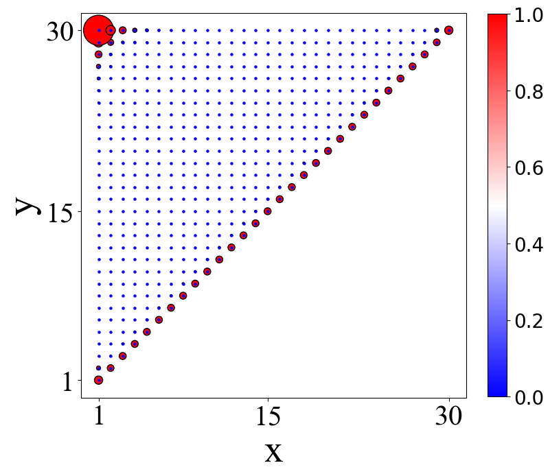
本征值为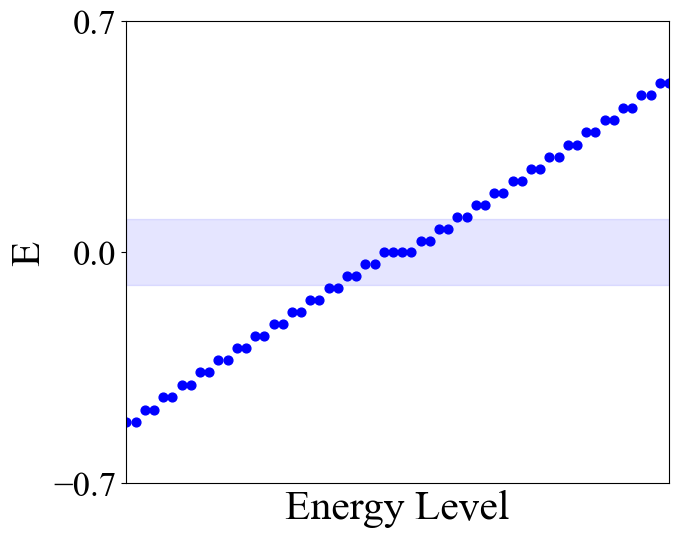
参考
鉴于该网站分享的大都是学习笔记,作者水平有限,若发现有问题可以发邮件给我
- yxliphy@gmail.com
也非常欢迎喜欢分享的小伙伴投稿


欢迎关注公众号,有趣的内容也会在上面同步。 有密码的文章属于正在建设中或者没有通过验证的内容,若有需要可通过邮件联系。