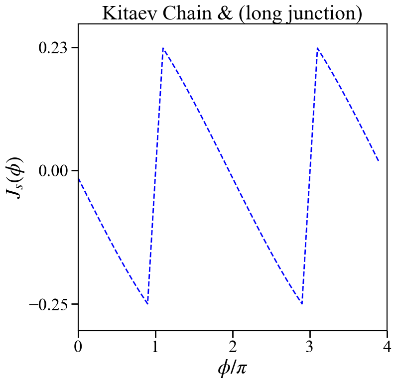
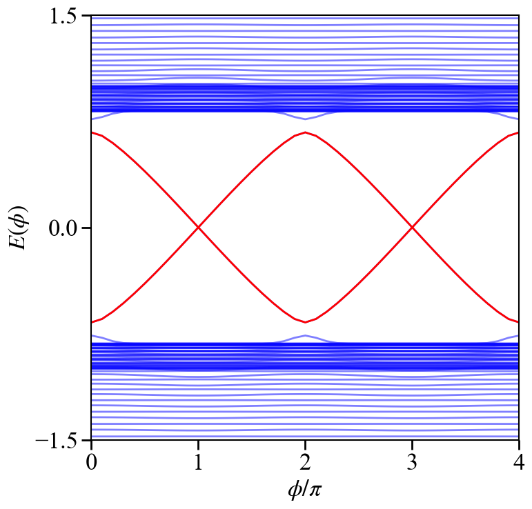
拓扑超导中存在Majorana费米子时,因为其满足非阿贝尔统计,会出现$4\pi$-Josephson效应。这里就研究Kitaev模型中的Josephson效应。
前言
这里是想实现一个有Kitaev模型构成的Josephson结,在结的两侧分别具有Majorana费米子,在中间加入一个绝缘体,从而系统中会存在零能Andreev束缚态,Josephson电流也会出现$4\pi$的周期。具体的物理内涵在这里先不解释了,我自己暂时对其中的内容理解不是很透彻,等之后完全理解了再重新整理一份笔记详细讨论关于拓扑超导体中的Josephson效应。
直接上代码计算Josephson效应
# 构造Josephson junction
@everywhere using SharedArrays, LinearAlgebra,Distributed,DelimitedFiles,Printf,Arpack
# --------------------------------------
@everywhere function pauli()
    s0 = zeros(ComplexF64,2,2)
    s1 = zeros(ComplexF64,2,2)
    s2 = zeros(ComplexF64,2,2)
    s3 = zeros(ComplexF64,2,2)
    #----
    s0[1,1] = 1
    s0[2,2] = 1
    #----
    s1[1,2] = 1
    s1[2,1] = 1
    #----
    s2[1,2] = -im
    s2[2,1] = im
    #-----
    s3[1,1] = 1
    s3[2,2] = -1
    #-----
    return s0,s1,s2,s3
end
#---------------------------------------------------------------
@everywhere function boundary(xn::Int64)
    bry = zeros(Int64,2,xn)
    for i0 in 1:xn
        bry[1,i0] = i0 + 1
        if i0 == xn
            bry[1,i0] = bry[1,i0] - xn
        end
        bry[2,i0] = i0 - 1
        if i0 == 1
            bry[2,i0] = bry[2,i0] + xn
        end
    end
    return bry
end
#-------------------------------------------------------------------
@everywhere function junction(ix::Int64,phil::Float64,phir::Float64,lpos::Int64,rpos::Int64)
    # 两侧超导位相存在差
    if ix <= lpos
        return exp(im*phil)
    elseif ix >= rpos
        return exp(im*phir)
    else
        return 0 # 正常态区域不存在电子配对,设置为零
    end
end
#-----------------------------------------------------------------------------------------
@everywhere function orpar1(ix::Int64,phil::Float64,phir::Float64,lpos::Int64,rpos::Int64)::Matrix{ComplexF64}
    # dx^2-y^2 pairing
    phi = junction(ix,phil,phir,lpos,rpos)
    g1 = zeros(ComplexF64,4,4)
    g1[1,2] = -im*phi
    g1[2,1] = conj(g1[1,2])
    return g1
end
#-----------------------------------------------------------------------------------------
@everywhere function matset(phil::Float64,phir::Float64,lpos::Int64,rpos::Int64)
    t0::Float64 = 1.0
    mu::Float64 = 1.0
    d0::Float64 = 1.0
    hn::Int64 = 2
    xn::Int64 = 100  # 开边界格点数量
    N::Int64 = xn*hn
    ham = zeros(ComplexF64,N,N)
    s0,sx,sy,sz = pauli()
    bry = boundary(xn)
    #------------------------
    for i0 in 1:xn
        g1 = orpar1(i0,phil,phir,lpos,rpos) # 需要对序参量进行修正
        for i1 in 0:hn - 1,i2 in 0:hn - 1
            ham[i0 + i1*xn,i0 + i2*xn] = -mu*sz[i1 + 1,i2 + 1]
            if i0 != xn
                ham[i0 + i1*xn,bry[1,i0] + i2*xn] = -t0*sz[i1 + 1,i2 + 1] + d0/(2*im)*g1[i1 + 1,i2 + 1]
            end
            if i0 != 1
                ham[i0 + i1*xn,bry[2,i0] + i2*xn] = -t0*sz[i1 + 1,i2 + 1] - d0/(2*im)*g1[i1 + 1,i2 + 1]
            end
        end
    end
    #-----------------------------------
    # 修正边界hopping
    for ix in 1:xn
        i0 = ix
        for i1 in 0:hn -1,i2 in 0:hn - 1
            if ix == lpos
                ham[i0 + xn * i1,bry[1,i0] + xn * i2] = -t0*sz[i1 + 1,i2 + 1]
            elseif ix == rpos
                ham[i0 + xn * i1,bry[2,i0] + xn * i2] = -t0*sz[i1 + 1,i2 + 1]
            end
        end
    end
    #-----------------
    if ~ishermitian(ham)
        f1 = open("hermi.dat","w")
        for m1 in 1:N,m2 in 1:N
            if ham[m1,m2] != conj(ham[m2,m1])
                # println("(",m1,",",m2,")",ham[m1,m2],ham[m2,m1])
                writedlm(f1,[real(m1) real(m2) ham[m1,m2] ham[m2, m1]],"\t")
            end
        end
        close(f1)
    end
    #-----------------------------------------
    if ishermitian(ham)
        temp2 = (a->(@sprintf "%3.1f" a)).(phir/pi)
        fx1 = "eigval-phase-" * temp2 * ".dat"
        #f1 = open(fx1,"w")
        val,vec = eigen(ham)
        # val,vec = eigs(ham,nev = 50,maxiter = 30,which = :SM)
        ind = (a->(@sprintf "%5.2f" a)).(range(1,length(val),length = length(val)))
        val2 = (a->(@sprintf "%15.8f" a)).(sort(map(real,val)))
        #writedlm(f1,[ind val2],"\t")
        #close(f1)
    else
        println("Hamiltonian is not hermitian")
        # break
    end
    return sort(map(real,val))
end
#--------------------------------------------------------------------------------
@everywhere function phase()
    philist = 0:0.1:4
    vallist = SharedArray(zeros(Float64,length(philist),200))
    @sync @distributed for i0 in 1:length(philist)
        vallist[i0,:] = matset(0.0,philist[i0]*pi,50,51)
    end
    fx1 = "KitaevChain-short.dat"
    f1 = open(fx1,"w")
    x0 = (a->(@sprintf "%15.8f" a)).(philist)
    y0 = (a->(@sprintf "%15.8f" a)).(vallist)
    writedlm(f1,[x0 y0],"\t")
end
#-----------------------------------------------------------------------------------
@everywhere function current()
    kbT::Float64 = 0.001
    dphi::Float64 = 0.1
    philist = 0:dphi:4
    vallist = SharedArray(zeros(Float64,length(philist),200))
    @sync @distributed for i0 in 1:length(philist)
        vallist[i0,:] = matset(0.0,philist[i0]*pi,50,51)
    end
    len1 = length(vallist[1,:]) # 只需要能量为正的本征值
    I0 = []
    phi = []
    for i0 in 1:length(philist) - 1 # loop for phase
        re1 = 0
        for i1 in Int(len1/2) + 1:len1 # loop for eigvals
            re1 += tanh(1/kbT*vallist[i0,i1]/2)*(vallist[i0 + 1,i1] - vallist[i0,i1])/(dphi*pi)
        end
        append!(I0,re1)
        append!(phi,philist[i0])
    end
    fx1 = "KitaevChain-current.dat"
    f1 = open(fx1,"w")
    x0 = (a->(@sprintf "%15.8f" a)).(phi)
    y0 = (a->(@sprintf "%15.8f" a)).(I0)
    writedlm(f1,[x0 y0],"\t")
    # writedlm(f1,[y0],"\t")
    close(f1)
end
#------------------------------------------------------------------------------------
@time phase()
@time current()
结果
这里分别计算了体系的能谱$E(\phi)$随着两侧超导位相差的变化以及Josephson电流$J_s(\phi)$。
绘图程序
习惯了用python进行绘图,这里顺便就把绘图程序也放在这里,方便自己平时查一些设置。
plot-$E(\phi)$
import numpy as np
import matplotlib.pyplot as plt
from matplotlib import rcParams
import os
config = {
"font.size": 30,
"mathtext.fontset":'stix',
"font.serif": ['SimSun'],
}
rcParams.update(config) # Latex 字体设置
#---------------------------------------------------------
def plotline(cont):
    # dataname = "m1-oy-" + str(cont).rjust(2,'0') + ".dat"
    dataname = "KitaevChain-short.dat"
    picname = os.path.splitext(dataname)[0] + ".png"
    os.chdir(os.getcwd())# 确定用户执行路径
    x0 = np.loadtxt(dataname)
    plt.figure(figsize=(8,8))
    plt.plot(x0[:,0], x0[:,1:int(len(x0[1,:])/2)], c = 'blue',alpha = 0.5,lw = 2)
    plt.plot(x0[:,0], x0[:,int(len(x0[1,:])/2) + 2:-1], c = 'blue',alpha = 0.5,lw = 2)
    #-----------
    plt.plot(x0[:,0], x0[:,int(len(x0[1,:])/2) -1], c = 'red',lw = 2)
    plt.plot(x0[:,0], x0[:,int(len(x0[1,:])/2) + 2], c = 'red',lw = 2)

    x0min = np.min(x0[:,0])
    x0max = np.max(x0[:,0])
    # y0min = np.min(x0[:,1])
    # y0max = np.max(x0[:,1])
    font2 = {'family': 'Times New Roman',
             'weight': 'normal',
             'size': 25,
             }
    plt.xlim(x0min,x0max)
    plt.ylim(-1.5,1.5)
    plt.xlabel(r'$\phi/\pi$',font2)
    plt.ylabel("$E(\phi)$",font2)
    #tit = "$h_x =" + str(cont) + "$"
    # plt.title(tit,font2)
    #plt.yticks(fontproperties='Times New Roman', size = 15)
    #plt.xticks(fontproperties='Times New Roman', size = 15)
    plt.xticks([0,1,2,3,4],fontproperties='Times New Roman', size = 25)
    plt.yticks([-1.5,0,1.5],fontproperties='Times New Roman', size = 25)
    plt.tick_params(axis='x',width = 2,length = 10)
    plt.tick_params(axis='y',width = 2,length = 10)
    ax = plt.gca()
    ax.spines["bottom"].set_linewidth(1.5)
    ax.spines["left"].set_linewidth(1.5)
    ax.spines["right"].set_linewidth(1.5)
    ax.spines["top"].set_linewidth(1.5)
    plt.savefig(picname, dpi = 100, bbox_inches = 'tight')
    plt.close()
#---------------------------------------------------------
def main():
    for i0 in range(1,12):
        scatterplot1(i0)
#---------------------------------------------------------
if __name__=="__main__":
    #main()
    # scatterplot1(1)
    plotline(1)
plot-current
import numpy as np
import matplotlib.pyplot as plt
from matplotlib import rcParams
import os
config = {
"font.size": 30,
"mathtext.fontset":'stix',
"font.serif": ['SimSun'],
}
rcParams.update(config) # Latex 字体设置
#---------------------------------------------------------
def scatterplot1(cont):
    # dataname = "m1-oy-" + str(cont).rjust(2,'0') + ".dat"
    tit = "Kitaev Chain & (long junction)"
    dataname = "KitaevChain-current.dat"
    picname = os.path.splitext(dataname)[0] + ".png"
    os.chdir(os.getcwd())# 确定用户执行路径
    x0 = np.loadtxt(dataname)
    plt.figure(figsize=(8,8))
    # plt.plot(x0[:,0], x0[:,1:-1], c = 'lightblue', alpha = 0.5)
    # plt.plot(x0[:,0], x0[:,1], c = 'lightblue', alpha = 0.5)
    plt.plot(x0[:,0], x0[:,1], c = 'blue',lw = 2.0,ls = "--")
    x0min = np.min(x0[:,0])
    x0max = np.max(x0[:,0])
    y0min = np.min(x0[:,1])
    y0max = np.max(x0[:,1])
    font2 = {'family': 'Times New Roman',
             'weight': 'normal',
             'size': 30,
             }
    plt.xlim(x0min,x0max)
    plt.ylim(y0min + y0min/5,y0max + y0max/5)
    plt.xlabel(r'$\phi/\pi$',font2)
    plt.ylabel("$J_s(\phi)$",font2)
    #tit = "$h_x =" + str(cont) + "$"
    plt.title(tit,font2)
    plt.xticks([0,1,2,3,4],fontproperties='Times New Roman', size = 25)
    plt.yticks([round(y0min,2),0,round(y0max,2)],fontproperties='Times New Roman', size = 25)
    plt.tick_params(axis='x',width = 2,length = 10)
    plt.tick_params(axis='y',width = 2,length = 10)
    ax = plt.gca()
    ax.spines["bottom"].set_linewidth(1.5)
    ax.spines["left"].set_linewidth(1.5)
    ax.spines["right"].set_linewidth(1.5)
    ax.spines["top"].set_linewidth(1.5)
    plt.savefig(picname, dpi = 100, bbox_inches = 'tight')
    plt.close()
#---------------------------------------------------------
def main():
    for i0 in range(1,12):
        scatterplot1(i0)
#---------------------------------------------------------
if __name__=="__main__":
    #main()
    scatterplot1(1)
公众号
相关内容均会在公众号进行同步,若对该Blog感兴趣,欢迎关注微信公众号。

|
yxli406@gmail.com |