几个简单模型的量子几何张量计算
前言
对于一个量子态$\lvert u(\mathbf{k}\rangle$,它的量子几何张量为
而量子几何张量的实部就是量子度规
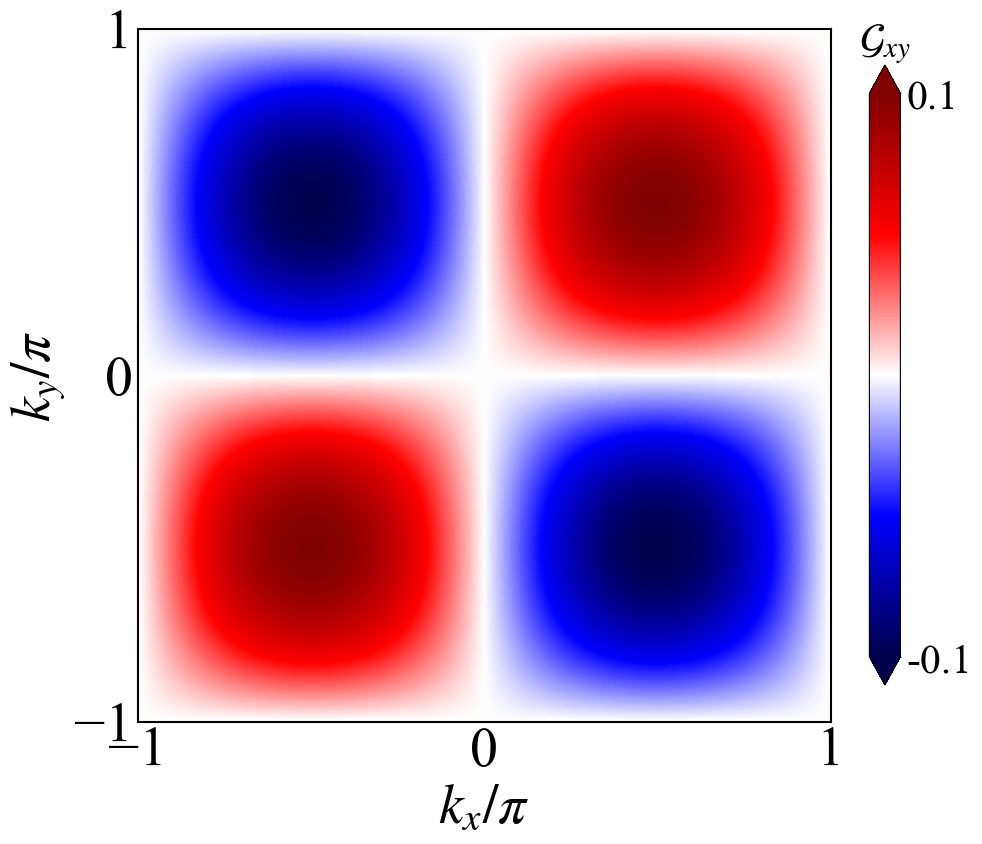
度规可调的平带模型
考虑一个拓扑平庸但是度规可调的平带模型
其中$\alpha(\mathbf{k})=\chi[\cos(k_x a)+\cos(k_y a)]$, $t_2$是最近邻跃迁大小,$\mu$是化学势,$s=\{ \uparrow,\downarrow \}$是自旋指标$s_z=\pm 1$。该哈密顿量具有时间反演对称性$h_{\uparrow}(\mathbf{k})=h^{*}_{\downarrow}(-\mathbf{k})$,其能带色散为
两个本征波函数为
结合前面两字几何张量的定义,将本征波函数代入可得
从而得到量子度规的解析表达式
下面就用代码实现以下1
2
3
4
5
6
7
8
9
10
11
12
13
14
15
16
17
18
19
20
21
22
23
24
25
26
27
28
29
30
31
32
33
34
35
36
37
38
39
40
41
42
43
44
45
46
47
48
49
50
51
52
53
54
55
56
57
58
59
60
61
62
63
64
65
66
67
68
69
70
71
72
73
74
75
76
77
78
79
80
81
82
83
84
85
86
87
88
89
90
91
92
93
94
95
96
97
98
99
100
101
102
103
104
105
106
107
108
109
110
111
112
113
114
115
116
117
118
119
120
121
122
123
124
125
126
127
128
129
130
131# ========================================================================================================================
# 计算给定模型的量子几何张量
# Ref: Anomalous Coherence Length in Superconductors with Quantum Metric(http://arxiv.org/abs/2308.05686)
# ========================================================================================================================
using SharedArrays,LinearAlgebra,Distributed,DelimitedFiles,Printf,BenchmarkTools,Arpack,Dates
#----------------------------------------------------------------------------------------------------------------------------
function PauliMatrix()
s0 = zeros(ComplexF64,2,2)
sx = zeros(ComplexF64,2,2)
sy = zeros(ComplexF64,2,2)
sz = zeros(ComplexF64,2,2)
s0[1,1] = 1
s0[2,2] = 1
sx[1,2] = 1
sx[2,1] = 1
sy[1,2] = -im
sy[2,1] = im
sz[1,1] = 1
sz[2,2] = -1
return s0,sx,sy,sz
end
#----------------------------------------------------------------------------------------------------------------------------
function matset(kx::Float64,ky::Float64)::Matrix
t0::Float64 = 1.0
mu::Float64 = 0.0
t2::Float64 = 0.0
chi::Float64 = 0.5
alpha::Float64 = 0.0
hn::Int64 = 2
Ham = zeros(ComplexF64,hn,hn)
alpha = chi * (cos(kx) + cos(ky))
s0,sx,sy,sz = PauliMatrix()
Ham = -t0 * (sin(alpha) * sx + cos(alpha) * sy) + (-2 * t2 * (cos(kx) + cos(ky)) - mu) * s0
return Ham
end
#----------------------------------------------------------------------------------------------------------------------------
function matset_dkxky(kx::Float64,ky::Float64)
# 计算哈密顿量的导数
hn::Int64 = 2
dk::Float64 = 1E-5
Ham = zeros(ComplexF64,hn,hn)
Hamdk = zeros(ComplexF64,hn,hn)
D_Ham = zeros(ComplexF64,2,hn,hn) # 哈密顿量偏导
# DH_kx
Ham = matset(kx - dk,ky)
Hamdk = matset(kx + dk,ky)
D_Ham[1,:,:] = (Hamdk - Ham)/(2.0 * dk)
# DH_ky
Ham = matset(kx,ky - dk)
Hamdk = matset(kx,ky + dk)
D_Ham[2,:,:] = (Hamdk - Ham)/(2.0 * dk)
return D_Ham
end
#----------------------------------------------------------------------------------------------------------------------------
function QGT_cal(kx::Float64,ky::Float64)
# 计算给定能带(bandindex)的量子几何张量(Qxx,Qxy,Qyx,Qyy)
eta::Float64 = 1E-5
ham = matset(kx,ky)
ham_dk = matset_dkxky(kx,ky)
vals,vecs = eigen(ham)
hn = size(ham)[1] # 根据哈密顿量来确定矩阵维度
re1 = zeros(ComplexF64,hn,2,2)
for mu in 1:2,nu in 1:2
for bandindex in 1:hn
for ie in 1:hn
if ie != bandindex
re1[bandindex,mu,nu] += ((vecs[:,bandindex]' * ham_dk[mu,:,:] * vecs[:,ie]) * (vecs[:,ie]' * ham_dk[nu,:,:] * vecs[:,bandindex]))/(vals[bandindex] - vals[ie] + eta)^2
end
end
end
end
return re1
end
#----------------------------------------------------------------------------------------------------------------------------
function QGT(bandindex::Int64)
kn::Int64 = 100
hn::Int64 = 2
klist = range(-pi,pi,length = kn)
kxlist = zeros(Float64,kn^2)
kylist = zeros(Float64,kn^2)
re1 = zeros(ComplexF64,kn^2,hn,2,2)
for ikx in 1:kn,iky in 1:kn
ik0 = Int((ikx - 1) * kn + iky)
kxlist[ik0] = klist[ikx]/pi
kylist[ik0] = klist[iky]/pi
re1[ik0,:,:,:] = QGT_cal(klist[ikx],klist[iky]) # 计算每个动量点上的QGT并存储
end
fx1 ="QGT.dat"
f1 = open(fx1,"w")
x0 = (a->( "%15.8f" a)).(kxlist)
y0 = (a->( "%15.8f" a)).(kylist)
z0 = (a->( "%15.8f" a)).(real(re1[:,bandindex,1,2]))
writedlm(f1,[x0 y0 z0],"\t")
close(f1)
return
end
#----------------------------------------------------------------------------------------------------------------------------
function QGT_parallel(bandindex::Int64)
kn::Int64 = 100
hn::Int64 = 2
klist = range(-pi,pi,length = kn)
kxlist = SharedArray(zeros(Float64,kn^2))
kylist = SharedArray(zeros(Float64,kn^2))
re1 = SharedArray(zeros(ComplexF64,kn^2,hn,2,2))
for ikx in 1:kn
for iky in 1:kn
ik0 = Int((ikx - 1) * kn + iky)
kxlist[ik0] = klist[ikx]/pi
kylist[ik0] = klist[iky]/pi
re1[ik0,:,:,:] = QGT_cal(klist[ikx],klist[iky]) # 计算每个动量点上的QGT并存储
end
end
fx1 ="QGT.dat"
f1 = open(fx1,"w")
x0 = (a->( "%15.8f" a)).(kxlist)
y0 = (a->( "%15.8f" a)).(kylist)
z0 = (a->( "%15.8f" a)).(real(re1[:,bandindex,1,2]))
writedlm(f1,[x0 y0 z0],"\t")
close(f1)
return
end
#----------------------------------------------------------------------------------------------------------------------------
function main()
return
end
#----------------------------------------------------------------------------------------------------------------------------
QGT(2)
绘图
1 | import numpy as np |
再给一下Mathematica计算的代码
1 | ClearAll["`*"] |
Lieb模型
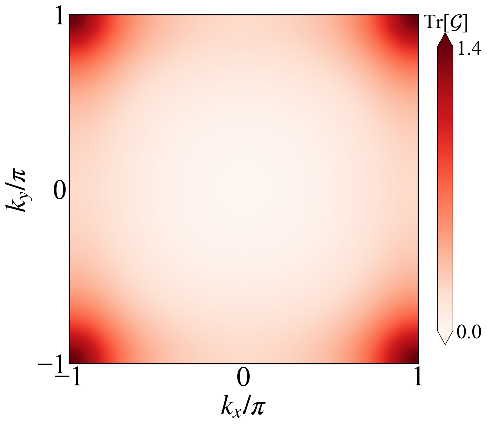
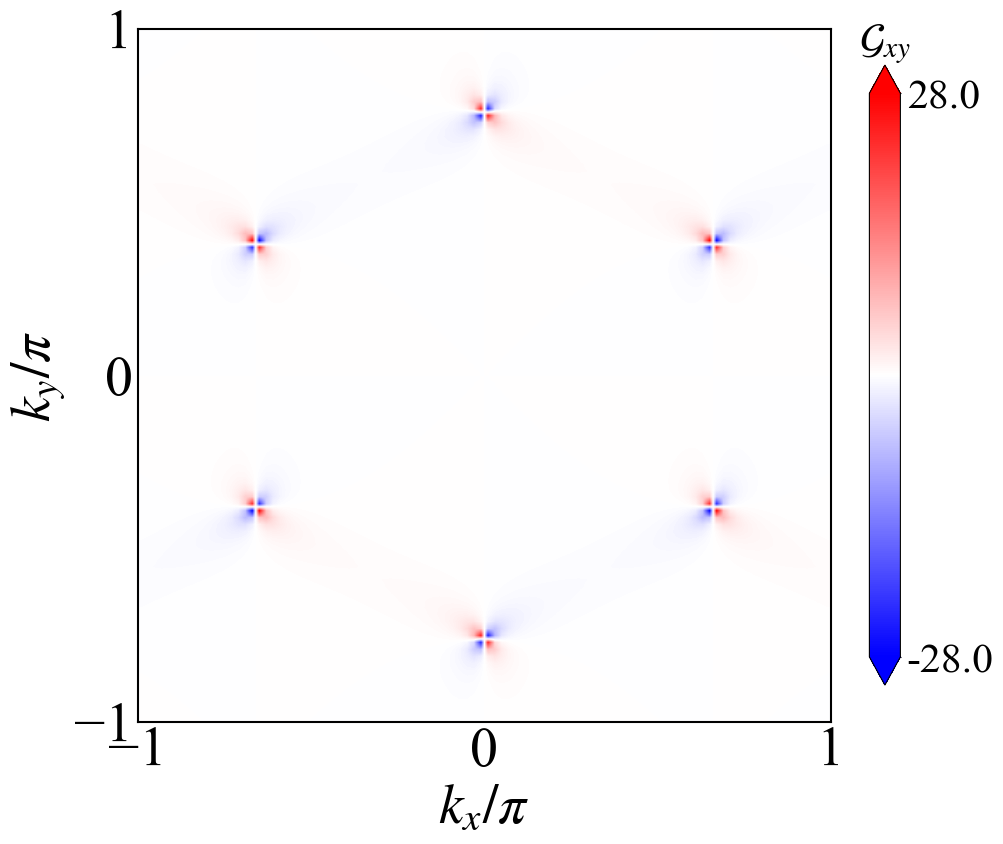
Lieb模型也具有一个平带,但是该模型可以是拓扑非平庸的,这里就只关注其度规部分。哈密顿量为
其中
这里给出Lieb模型量子几何张量实部量子度规的计算1
2
3
4
5
6
7
8
9
10
11
12
13
14
15
16
17
18
19
20
21
22
23
24
25
26
27
28
29
30
31
32
33
34
35
36
37
38
39
40
41
42
43
44
45
46
47
48
49
50
51
52
53
54
55
56
57
58
59
60
61
62
63
64
65
66
67
68
69
70
71
72
73
74
75
76
77
78
79
80
81
82
83
84
85
86
87
88
89
90
91
92
93
94
95
96
97
98
99
100
101
102
103
104
105
106
107
108
109
110
111
112
113
114
115
116
117
118# ========================================================================================================================
# 计算Lieb模型的量子几何张量
# Ref: Anomalous Coherence Length in Superconductors with Quantum Metric(http://arxiv.org/abs/2308.05686)
# ========================================================================================================================
using SharedArrays,LinearAlgebra,Distributed,DelimitedFiles,Printf,BenchmarkTools,Arpack,Dates
#----------------------------------------------------------------------------------------------------------------------------
function matset(kx::Float64,ky::Float64)::Matrix
J0::Float64 = 1.0
t2::Float64 = 0.0
eta::Float64 = 0.3 * J0
hn::Int64 = 3
Ham = zeros(ComplexF64,hn,hn)
fx = 2 * J0 * (cos(kx/2.0) + im * eta * sin(kx/2.0))
fy = 2 * J0 * (cos(ky/2.0) + im * eta * sin(ky/2.0))
f2 = 2 * t2 * (cos((kx + ky)/2.0) + cos((kx - ky)/2.0))
Ham[1,2] = fx
Ham[1,3] = f2
Ham[2,1] = fx'
Ham[2,3] = fy
Ham[3,1] = f2'
Ham[3,2] = fy'
return Ham
end
#----------------------------------------------------------------------------------------------------------------------------
function matset_dkxky(hn::Int64,kx::Float64,ky::Float64)
# 计算哈密顿量的导数
dk::Float64 = 1E-5
Ham = zeros(ComplexF64,hn,hn)
Hamdk = zeros(ComplexF64,hn,hn)
D_Ham = zeros(ComplexF64,2,hn,hn) # 哈密顿量偏导
# DH_kx
Ham = matset(kx - dk,ky)
Hamdk = matset(kx + dk,ky)
D_Ham[1,:,:] = (Hamdk - Ham)/(2.0 * dk)
# DH_ky
Ham = matset(kx,ky - dk)
Hamdk = matset(kx,ky + dk)
D_Ham[2,:,:] = (Hamdk - Ham)/(2.0 * dk)
return D_Ham
end
#----------------------------------------------------------------------------------------------------------------------------
function QGT_cal(kx::Float64,ky::Float64)
# 计算给定能带(bandindex)的量子几何张量(Qxx,Qxy,Qyx,Qyy)
eta::Float64 = 1E-5
ham = matset(kx,ky)
hn = size(ham)[1] # 根据哈密顿量来确定矩阵维度
ham_dk = matset_dkxky(hn,kx,ky)
vals,vecs = eigen(ham)
re1 = zeros(ComplexF64,hn,2,2)
for mu in 1:2,nu in 1:2
for bandindex in 1:hn
for ie in 1:hn
if ie != bandindex
re1[bandindex,mu,nu] += ((vecs[:,bandindex]' * ham_dk[mu,:,:] * vecs[:,ie]) * (vecs[:,ie]' * ham_dk[nu,:,:] * vecs[:,bandindex]))/(vals[bandindex] - vals[ie] + eta)^2
end
end
end
end
return re1
end
#----------------------------------------------------------------------------------------------------------------------------
function QGT(bandindex::Int64)
kn::Int64 = 100
ham = matset(0.1,0.1)
hn = size(ham)[1] # 根据哈密顿量来确定矩阵维度
klist = range(-pi,pi,length = kn)
kxlist = zeros(Float64,kn^2)
kylist = zeros(Float64,kn^2)
re1 = zeros(ComplexF64,kn^2,hn,2,2)
for ikx in 1:kn,iky in 1:kn
ik0 = Int((ikx - 1) * kn + iky)
kxlist[ik0] = klist[ikx]/pi
kylist[ik0] = klist[iky]/pi
re1[ik0,:,:,:] = QGT_cal(klist[ikx],klist[iky]) # 计算每个动量点上的QGT并存储
end
fx1 ="QGT-lieb.dat"
f1 = open(fx1,"w")
x0 = (a->( "%15.8f" a)).(kxlist)
y0 = (a->( "%15.8f" a)).(kylist)
z0 = (a->( "%15.8f" a)).(real(re1[:,bandindex,1,1] + re1[:,bandindex,2,2]))
writedlm(f1,[x0 y0 z0],"\t")
close(f1)
return
end
#----------------------------------------------------------------------------------------------------------------------------
function QGT_parallel(bandindex::Int64)
kn::Int64 = 100
hn::Int64 = 2
klist = range(-pi,pi,length = kn)
kxlist = SharedArray(zeros(Float64,kn^2))
kylist = SharedArray(zeros(Float64,kn^2))
re1 = SharedArray(zeros(ComplexF64,kn^2,hn,2,2))
for ikx in 1:kn
for iky in 1:kn
ik0 = Int((ikx - 1) * kn + iky)
kxlist[ik0] = klist[ikx]/pi
kylist[ik0] = klist[iky]/pi
re1[ik0,:,:,:] = QGT_cal(klist[ikx],klist[iky]) # 计算每个动量点上的QGT并存储
end
end
fx1 ="QGT-lieb.dat"
f1 = open(fx1,"w")
x0 = (a->( "%15.8f" a)).(kxlist)
y0 = (a->( "%15.8f" a)).(kylist)
z0 = (a->( "%15.8f" a)).(real(re1[:,bandindex,1,2]))
writedlm(f1,[x0 y0 z0],"\t")
close(f1)
return
end
#----------------------------------------------------------------------------------------------------------------------------
function main()
return
end
#----------------------------------------------------------------------------------------------------------------------------
QGT(2) # 第二条能带是平带
Graphene Quantum Metric
1 | # ======================================================================================================================== |
Sawtooth模型
Sawtooth模型的晶格结构如下图所示
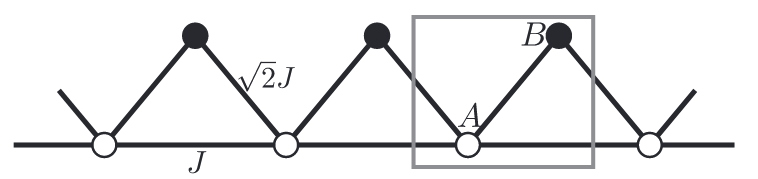
每个原胞内有两个轨道$(A,B)$,其哈密顿量为
该模型两个能带的度规是相同的
下面直接上数值计算的代码了1
2
3
4
5
6
7
8
9
10
11
12
13
14
15
16
17
18
19
20
21
22
23
24
25
26
27
28
29
30
31
32
33
34
35
36
37
38
39
40
41
42
43
44
45
46
47
48
49
50
51
52
53
54
55
56
57
58
59
60
61
62
63
64
65
66
67
68
69
70
71
72
73
74# ========================================================================================================================
# 计算Sawthhod 模型的量子度规
# Ref: Wave-packet dynamics of Bogoliubov quasiparticles: Quantum metric effects(https://link.aps.org/doi/10.1103/PhysRevB.96.064511)
# ========================================================================================================================
using SharedArrays,LinearAlgebra,Distributed,DelimitedFiles,Printf,BenchmarkTools,Arpack,Dates
#----------------------------------------------------------------------------------------------------------------------------
function matset(kx::Float64,)::Matrix
J0::Float64 = 1.0
mu::Float64 = -2
hn::Int64 = 2
Ham = zeros(ComplexF64,hn,hn)
Ham[1,1] = 2 * J0 * cos(kx) - mu
Ham[1,2] = 2 * J0 * cos(kx/2.0)
Ham[2,1] = 2 * J0 * cos(kx/2.0)
Ham[2,2] = -mu
return Ham
end
#----------------------------------------------------------------------------------------------------------------------------
function matset_dkxky(hn::Int64,kx::Float64)
# 计算哈密顿量的导数
dk::Float64 = 1E-5
Ham = zeros(ComplexF64,hn,hn)
Hamdk = zeros(ComplexF64,hn,hn)
D_Ham = zeros(ComplexF64,hn,hn) # 哈密顿量偏导
# DH_kx
Ham = matset(kx - dk)
Hamdk = matset(kx + dk)
D_Ham = (Hamdk - Ham)/(2.0 * dk)
return D_Ham
end
#----------------------------------------------------------------------------------------------------------------------------
function QGT_cal(kx::Float64,)
# 计算给定能带(bandindex)的量子几何张量(Qxx)
eta::Float64 = 1E-3
ham = matset(kx)
hn = size(ham)[1] # 根据哈密顿量来确定矩阵维度
ham_dk = matset_dkxky(hn,kx)
vals,vecs = eigen(ham)
re1 = zeros(ComplexF64,hn)
for bandindex in 1:hn
for ie in 1:hn
if ie != bandindex
re1[bandindex] += ((vecs[:,bandindex]' * ham_dk * vecs[:,ie]) * (vecs[:,ie]' * ham_dk * vecs[:,bandindex]))/(vals[bandindex] - vals[ie] + eta)^2
end
end
end
return re1
end
#----------------------------------------------------------------------------------------------------------------------------
function QGT(bandindex::Int64)
kn::Int64 = 2E2
ham = matset(0.1)
hn = size(ham)[1] # 根据哈密顿量来确定矩阵维度
klist = range(-pi,pi,length = kn)
re1 = SharedArray(zeros(ComplexF64,kn,hn))
re2 = SharedArray(zeros(Float64,kn))
for ikx in 1:kn
kx = klist[ikx]/pi
re1[ikx,:] = QGT_cal(kx) # 计算每个动量点上的QGT并存储
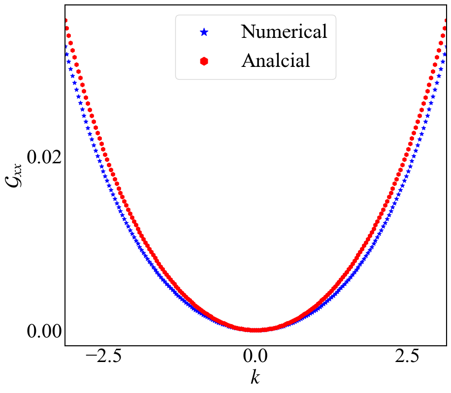
re2[ikx] = (1 - cos(kx))/(2(2 + cos(kx))^2) # 解析结果
end
fx1 ="QGT-Sawthhod.dat"
f1 = open(fx1,"w")
x0 = (a->( "%15.8f" a)).(klist)
z0 = (a->( "%15.8f" a)).(real(re1[:,bandindex]))
z1 = (a->( "%15.8f" a)).(imag(re1[:,bandindex]))
z2 = (a->( "%15.8f" a)).(real(re2))
writedlm(f1,[x0 z0 z1 z2],"\t")
close(f1)
return
end
#----------------------------------------------------------------------------------------------------------------------------
QGT(1)
绘图代码1
2
3
4
5
6
7
8
9
10
11
12
13
14
15
16
17
18
19
20
21
22
23
24
25
26
27
28
29
30
31
32
33
34
35
36
37
38
39
40
41
42
43
44
45
46
47
48
49
50
51
52import numpy as np
import matplotlib.pyplot as plt
from matplotlib import rcParams
import os
import matplotlib.gridspec as gridspec
from matplotlib.path import Path
import matplotlib.colors as mcolors
plt.rc('font', family='Times New Roman')
config = {
"font.size": 30,
"mathtext.fontset":'stix',
"font.serif": ['SimSun'],
}
rcParams.update(config) # Latex 字体设置
#---------------------------------------------------------------------------------------------------------------------------------------------------------
def plot_QGT_Sawthhod():
dataname = "QGT-Sawthhod.dat"
picname = os.path.splitext(dataname)[0] + ".png"
da = np.loadtxt(dataname)
# 使用第一列和第二列分别作为 kx 和 ky
x0 = da[:, 0]
y0 = da[:, 1] # Quantum Metric numerical
y1 = da[:, 3] # Quantum Metric analy
plt.figure(figsize=(10, 9))
num_ticks = 3
Umax = np.max(da[:,0])
Umin = np.min(da[:,0])
plt.scatter(x0,y0,c = "b", marker = "*", label = r"Numerical")
plt.scatter(x0,y1,c = "r", marker = "h", label = r"Analcial")
plt.xlabel(r"$k$")
plt.ylabel(r"$\mathcal{G}_{xx}$")
plt.xlim(Umin,Umax)
plt.tick_params(direction = 'in' ,axis = 'x',width = 0,length = 10)
plt.tick_params(direction = 'in' ,axis = 'y',width = 0,length = 10)
plt.legend(loc='best', fontsize = 30, markerscale = 2)
# plt.axis('scaled')
ax = plt.gca()
ax.spines["bottom"].set_linewidth(1.5)
ax.spines["left"].set_linewidth(1.5)
ax.spines["right"].set_linewidth(1.5)
ax.spines["top"].set_linewidth(1.5)
ax.locator_params(axis='x', nbins = num_ticks) # x 轴最多显示 3 个刻度
ax.locator_params(axis='y', nbins = num_ticks) # y 轴最多显示 3 个刻度
# plt.show()
plt.savefig(picname, dpi = 100,bbox_inches = 'tight')
plt.close()
数值结果与解析结果对比
参考文献
- Anomalous Coherence Length in Superconductors with Quantum Metric
- Wave-packet dynamics of Bogoliubov quasiparticles: Quantum metric effects
鉴于该网站分享的大都是学习笔记,作者水平有限,若发现有问题可以发邮件给我
- yxliphy@gmail.com
也非常欢迎喜欢分享的小伙伴投稿


欢迎关注公众号,有趣的内容也会在上面同步。 有密码的文章属于正在建设中或者没有通过验证的内容,若有需要可通过邮件联系。