Kwant如何搞拓扑
边界态
先导入一波预设1
2
3
4
5
6
7
8
9
10
11
12
13
14
15
16
17
18
19
20
21
22
23
24
25
26
27
28
29
30
31
32
33
34
35
36
37
38
39
40
41
42
43
44
45
46
47
48
49
50
51
52import numpy as np,matplotlib,kwant,time,kwant.continuum,tinyarray
from matplotlib import pyplot as plt
from matplotlib.colors import LinearSegmentedColormap
from matplotlib.ticker import MaxNLocator
import scipy.sparse.linalg as sla # 本征值求解
# from Kwant.qw import lattice
matplotlib.use('MacOSX') # 或者选择其他可用的 backend(避免使用kwant视图出现报错)
# matplotlib.use('module://backend_interagg') # 使用嵌入式模式
# 调整全局绘图设置
plt.rcParams['text.usetex'] = True
plt.rcParams['font.family'] = 'Times New Roman' # 字体样式
plt.rcParams['figure.dpi'] = 300 # 全局设置保存图片分辨率
plt.rcParams['font.size'] = 30 # 设置字体大小为16
plt.rcParams['xtick.direction'] = 'in'
plt.rcParams['ytick.direction'] = 'in'
plt.rcParams['xtick.major.size'] = 4
plt.rcParams['ytick.major.size'] = 4
plt.rcParams['xtick.major.width'] = 1
plt.rcParams['ytick.major.width'] = 1
plt.rcParams['axes.linewidth'] = 1.5
s0 = tinyarray.array([[1, 0], [0, 1]])
sx = tinyarray.array([[0, 1], [1, 0]])
sy = tinyarray.array([[0, -1j], [1j, 0]])
sz = tinyarray.array([[1, 0], [0, -1]])
#------------------------------------------------------------------------------------------------
def sorted_eigs(eigs_result):
evals, evecs = eigs_result
idx = np.argsort(evals.real) # 只按实部排序(一般能量是实数)
return evals[idx], evecs[:, idx]
#------------------------------------------------------------------------------------------------
def plot_wave_function(syst, B=0.001):
ham_mat = syst.hamiltonian_submatrix(sparse=True, params=dict(B=B)) # 直接获取构建系统的哈密顿量
evals, evecs = sorted_eigs(sla.eigsh(ham_mat.tocsc(), k = 10, sigma=0)) # 这里只求解20个本征值,加速
# 绘制某一个能级对应的波函数在系统中的分布,show = False的时候才可以正确保存图片
fig, ax = plt.subplots(figsize=(12, 12)) # 先创建 figure 和 axes
fig = kwant.plotter.map(syst, np.abs(evecs[:, 9])**2,ax = ax, oversampling = 1,cmap = Make_color("TemperatureMap.dat"),show = False)
plt.savefig("close-wave.png", dpi=100, bbox_inches='tight')
plt.close(fig)
#------------------------------------------------------------------------------------------------
def plot_current(syst, B=0.001):
ham_mat = syst.hamiltonian_submatrix(sparse=True, params=dict(B=B)) # kwant默认构建出的是稀疏矩阵,是按行存储的(CRS),这样做矩阵运算的时候比较快
evals, evecs = sorted_eigs(sla.eigsh(ham_mat.tocsc(), k=20, sigma=0)) # 在对角化的时候将系数矩阵按列存储(CSC),这样对角化的时候更快
J = kwant.operator.Current(syst) # 获取系统的电流算符
current = J(evecs[:, 9], params = dict(B = B)) # 给定本征矢量计算出对应的电流分布
# 假设你已经有 syst 和 current 矩阵
fig, ax = plt.subplots(figsize=(12, 12)) # 先创建 figure 和 axes
# kwant.plotter.current(syst, current, ax=ax, cmap = Make_color("TemperatureMap.dat"), show=False,colorbar = True)
kwant.plotter.current(syst, current, ax=ax, show=False,colorbar = True)
plt.savefig("close-current.png", dpi=100, bbox_inches='tight')
plt.close(fig)
画个边界态看看1
2
3
4
5
6
7
8
9
10
11
12
13
14
15
16
17
18
19
20
21
22
23
24
25
26
27
28
29
30
31
32
33
34
35
36
37
38
39
40
41
42#------------------------------------------------------------------------------------------------
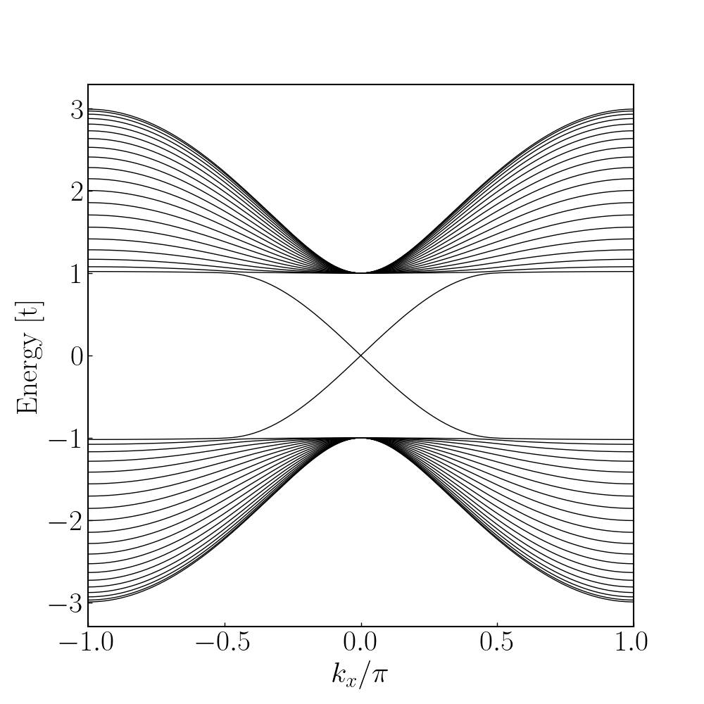
def Half_BHZ():
s0 = tinyarray.array([[1, 0], [0, 1]])
sx = tinyarray.array([[0, 1], [1, 0]])
sy = tinyarray.array([[0, -1j], [1j, 0]])
sz = tinyarray.array([[1, 0], [0, -1]])
m0 = 1.0;tx = 1.0;ty = 1.0;W0 = 20;ax = 1.0;ay = 1.0;a0 = 1.0;
lat = kwant.lattice.square(a0, norbs = 2)
sym_lead = kwant.TranslationalSymmetry((-a0, 0)) # 电极沿x方向是周期的
bhz = kwant.Builder(sym_lead)
for j in range(W0): # y方向占位
bhz[lat(0, j)] = m0 * sz
if j > 0: # 电极y方向hopping设置
bhz[lat(0, j), lat(0, j - 1)] = -ty/2.0 * sz - 1j * ay/2.0 * sy
bhz[lat(1, j), lat(0, j)] = -tx/2.0 * sz - 1j * ax/2.0 * sx
bhz = bhz.finalized()
# 可以选择调用系统函数绘制能带
# plt.figure(figsize = (10,10))
# kwant.plotter.bands(bhz, show=False)
# plt.xlabel(r"$k_x$")
# plt.ylabel(r"energy [t]")
# plt.savefig("half-bhz-cylinder.png",dpi = 100)
# 也可以用 kwant.physics.Bands 得到一个可调用对象,自己绘制能带图
bands = kwant.physics.Bands(bhz)
# 在某个 k 范围取样
ks = np.linspace(-np.pi, np.pi, 201) # kx 采样点
energies = [bands(k) for k in ks] # energies 是二维数组,每个 k 对应多个能带
energies = np.array(energies) # shape (len(ks), n_bands)
# 画图(你自己完全控制线条样式)
plt.figure(figsize=(10, 10))
for band in energies.T: # 按列画,每一列是一条能带
plt.plot(ks/np.pi, band, color = "k", lw = 1)
plt.xlabel(r"$k_x/\pi$")
plt.ylabel("Energy [t]")
plt.xlim(-1,1)
# plt.show()
plt.savefig("half-bhz-cylinder.png",dpi = 100)
plt.close()
计算电流分布和波函数分布1
2
3
4
5
6
7
8
9
10
11
12
13
14
15
16
17
18
19
20
21
22
23
24
25
26
27
28
29
30#------------------------------------------------------------------------------------------------
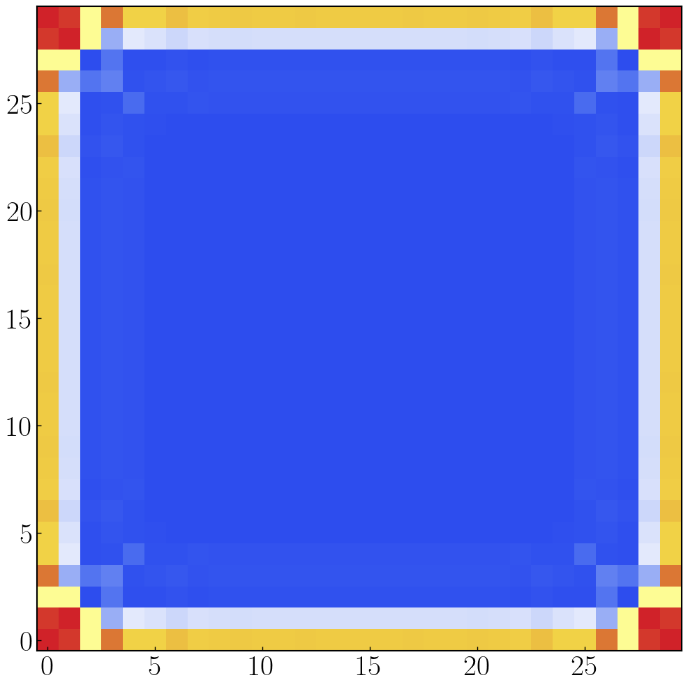
def half_bhz_current():
a0 = 1.0;M0 = 1.0;t0 = 1.0;A0 = 1.0;L0 = 30;W0 = L0;
bhz = kwant.Builder()
lattice = kwant.lattice.square(a0,norbs = 2)
bhz[(lattice(ix, iy) for ix in range(L0) for iy in range(W0))] = M0 * sz # 占位能设置
# 设置自旋轨道耦合,此时x方向和y方向具有差异性,每个方向都需要声明跃迁矩阵元
bhz[kwant.builder.HoppingKind((1, 0), lattice, lattice)] = -t0 * sz + 1j * A0 * sy / 2.0 # x方向跃迁
bhz[kwant.builder.HoppingKind((0, 1), lattice, lattice)] = -t0 * sz - 1j * A0 * sx / 2.0 # y方向跃迁
bhz = bhz.finalized()
ham_mat = bhz.hamiltonian_submatrix(sparse=True) # 直接获取构建系统的哈密顿量
num_vals = 30;
evals, evecs = sorted_eigs(sla.eigsh(ham_mat.tocsc(), k = num_vals, sigma=0)) # 这里只求解20个本征值,加速
# 绘制某一个能级对应的波函数在系统中的分布,show = False的时候才可以正确保存图片
fig, ax = plt.subplots(figsize=(12, 12)) # 先创建 figure 和 axes
wf = np.abs(evecs[:, int(num_vals/2)]) ** 2
wf_site = wf.reshape((-1, 2)).sum(axis=1) # 对每个格点的两个轨道求和
fig = kwant.plotter.map(bhz, wf_site, ax=ax,cmap=Make_color("TemperatureMap.dat"), show=False) # 绘制波函数分布
plt.savefig("half-bhz-wave.png", dpi=100, bbox_inches='tight')
plt.close(fig)
# plt.scatter(range(10),evals)
# plt.show()
J = kwant.operator.Current(bhz) # 获取系统的电流算符
current = J(evecs[:, int(num_vals/2)]) # 给定本征矢量计算出对应的电流分布
# 假设你已经有 syst 和 current 矩阵
fig, ax = plt.subplots(figsize=(12, 12)) # 先创建 figure 和 axes
fig = kwant.plotter.current(bhz, current, ax=ax, cmap = Make_color("TemperatureMap.dat"), show=False,colorbar = True)
# kwant.plotter.current(bhz, current, ax=ax, show=False, colorbar=True)
plt.savefig("half-bhz-current.png", dpi=100, bbox_inches='tight')
plt.close(fig)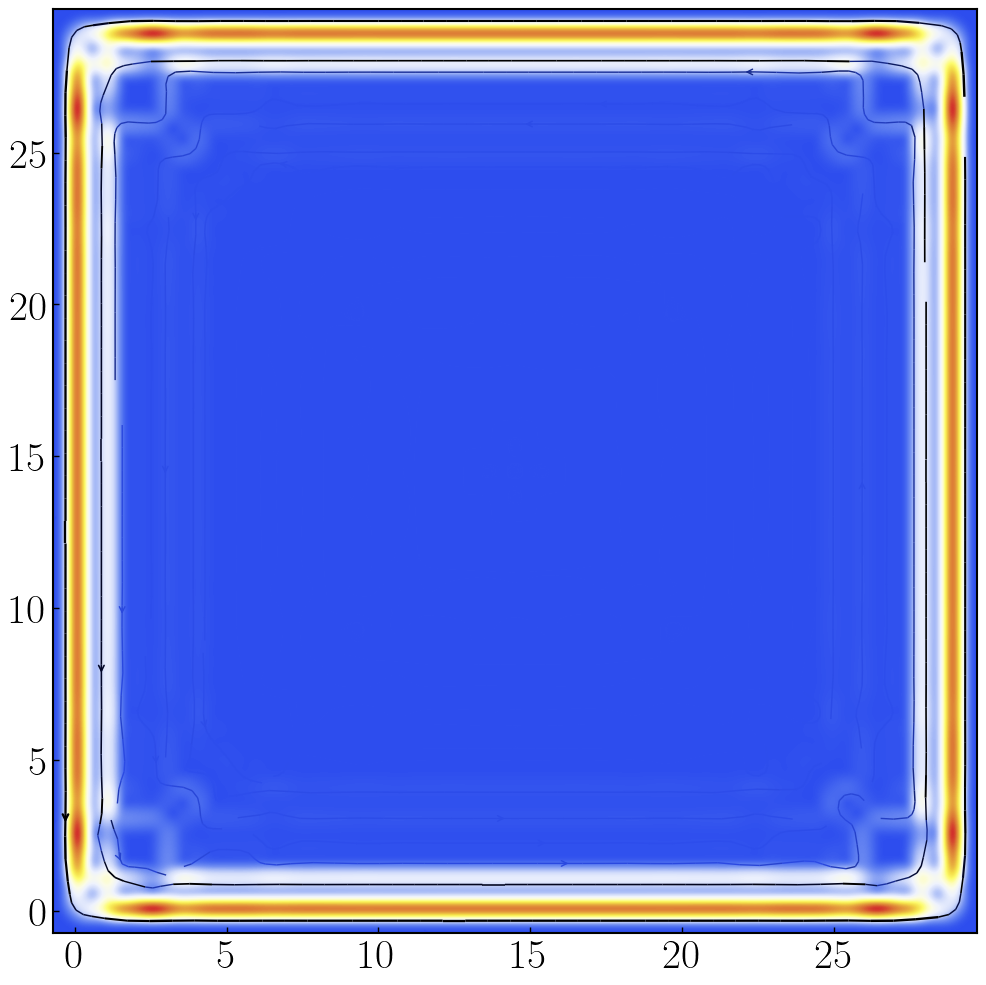
Kitaev模型
1 | def Kitaev_model(): |
高阶拓扑
1 | def HOTSC(): |
还可以构建不同形状的结构1
2
3
4
5
6
7
8
9
10
11
12
13
14
15
16
17
18
19
20
21
22
23
24
25
26
27
28
29
30
31
32
33
34
35
36
37
38
39
40
41
42
43
44
45
46
47
48
49
50
51
52
53
54
55
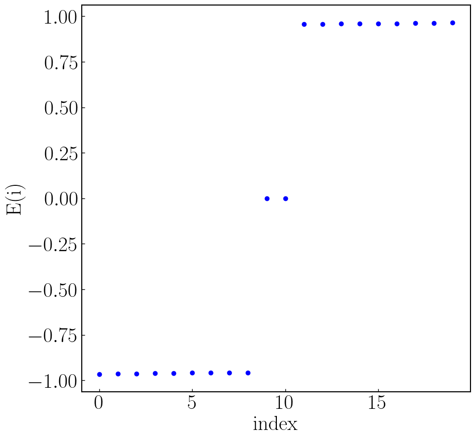
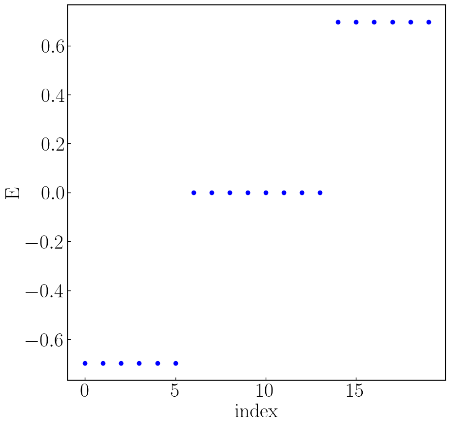
56def HOTSC_Ring():
a0 = 1.0;M0 = 1.0;t0 = 1.0;A0 = 1.0;delta0 = 0.5;L0 = 80;W0 = L0;orbits = 8;r0 = L0
hotsc = kwant.Builder()
lattice = kwant.lattice.square(a0, norbs = orbits)
# 限制一个圆形结构
def circle(pos):
(x, y) = pos
rsq = x ** 2 + y ** 2
return rsq < r0 ** 2
hotsc[lattice.shape(circle, (0, 0))] = M0 * np.kron(np.kron(sz, s0),sz) # 占位能设置(particle * spin * orbit)
# 设置自旋轨道耦合,此时x方向和y方向具有差异性,每个方向都需要声明跃迁矩阵元
hotsc[kwant.builder.HoppingKind((1, 0), lattice, lattice)] = -t0 * np.kron(np.kron(sz, s0), sz) \
+ 1j * A0 * np.kron(np.kron(s0, sz), sx) / 2.0 \
+ delta0 / 2.0 * np.kron(np.kron(sy, sy), s0) # x方向跃迁
hotsc[kwant.builder.HoppingKind((0, 1), lattice, lattice)] = -t0 * np.kron(np.kron(sz, s0), sz) \
- 1j * A0 * np.kron(np.kron(sz, s0), sy) / 2.0 \
- delta0 / 2.0 * np.kron(np.kron(sy, sy), s0) # y方向跃迁
hotsc = hotsc.finalized()
ham_mat = hotsc.hamiltonian_submatrix(sparse=True) # 直接获取构建系统的哈密顿量
num_vals = 50;
evals, evecs = sorted_eigs(sla.eigsh(ham_mat.tocsc(), k=num_vals, sigma=0)) # 这里只求解20个本征值,加速
fig, ax = plt.subplots(figsize=(10, 10)) # 先创建 figure 和 axes
plt.scatter(range(num_vals), evals, c="blue") # 绘制本征值
plt.xlabel(r"index");plt.ylabel(r"E")
ax = plt.gca()
ax.locator_params(axis='y', nbins=3) # y 轴最多显示 3 个刻度
ax.locator_params(axis='x', nbins=3) # y 轴最多显示 3 个刻度
# plt.show()
plt.savefig("hotsc-vals-circle.png", dpi=100, bbox_inches='tight')
plt.close()
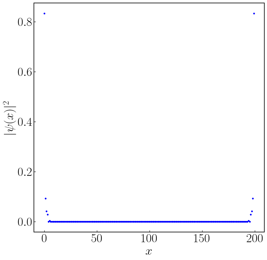
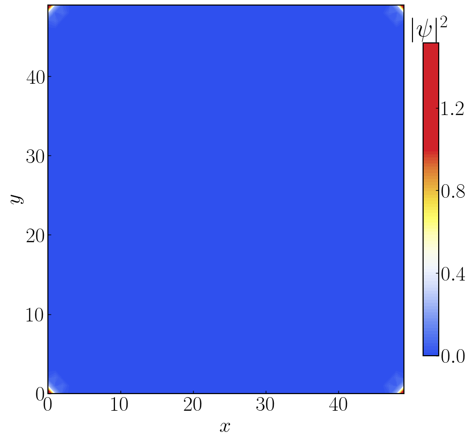
sites = hotsc.sites # 返回一个列表,每个元素就是一个 site
coords = np.array([site.pos for site in sites])
# 找到最接近零能量的本征值索引
tol = 1e-3 # 判定为“零能量”的阈值
zero_indices = np.where(np.abs(evals) < tol)[0]
wf = np.sum(np.array([np.abs(evecs[:, i0])**2 for i0 in zero_indices]), axis = 0)
wf_site = wf.reshape((-1, orbits)).sum(axis = 1) # 如果每个格点有多个轨道,需要先对轨道求和
plt.figure(figsize=(10, 10)) # 先创建 figure 和 axes
# cf = plt.scatter(coords[:, 0], coords[:, 1], c = wf_site, s = 15, cmap = Make_color("TemperatureMap.dat"))
cf = plt.scatter(coords[:, 0], coords[:, 1], c=wf_site, s=15, cmap = "magma_r")
cb = plt.colorbar(cf, fraction = 0.04, extend = 'both')
cb.locator = MaxNLocator(nbins = 5) # 最多显示 5 个刻度 # 设置刻度稀疏
cb.update_ticks()
cb.ax.tick_params(direction = 'in', labelsize = 30) # 设置colorbar的刻度向内
cb.ax.set_title(r"$|\psi|^2$")
plt.xlabel(r"$x$")
plt.ylabel(r"$y$")
plt.axis('equal') # 保持圆形比例
ax = plt.gca()
ax.locator_params(axis='y', nbins=3) # y 轴最多显示 3 个刻度
ax.locator_params(axis='x', nbins=3) # y 轴最多显示 3 个刻度
# plt.show()
plt.savefig("hotsc-wave-circle.png", dpi=100, bbox_inches='tight')
plt.close()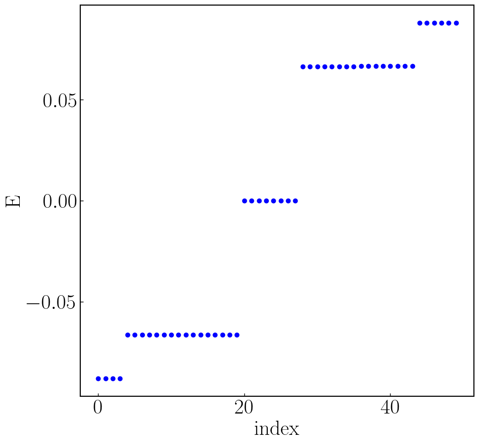

用Kwant计算有个便捷之处,它的矩阵存储使用的是稀疏矩阵方法,对角化的时候如果求解少量本征值也是在稀疏矩阵的基础上做的,因此可以把系统的尺寸取的相对大一些,而且计算速度还可以.
鉴于该网站分享的大都是学习笔记,作者水平有限,若发现有问题可以发邮件给我
- yxliphy@gmail.com
也非常欢迎喜欢分享的小伙伴投稿


欢迎关注公众号,有趣的内容也会在上面同步。 有密码的文章属于正在建设中或者没有通过验证的内容,若有需要可通过邮件联系。