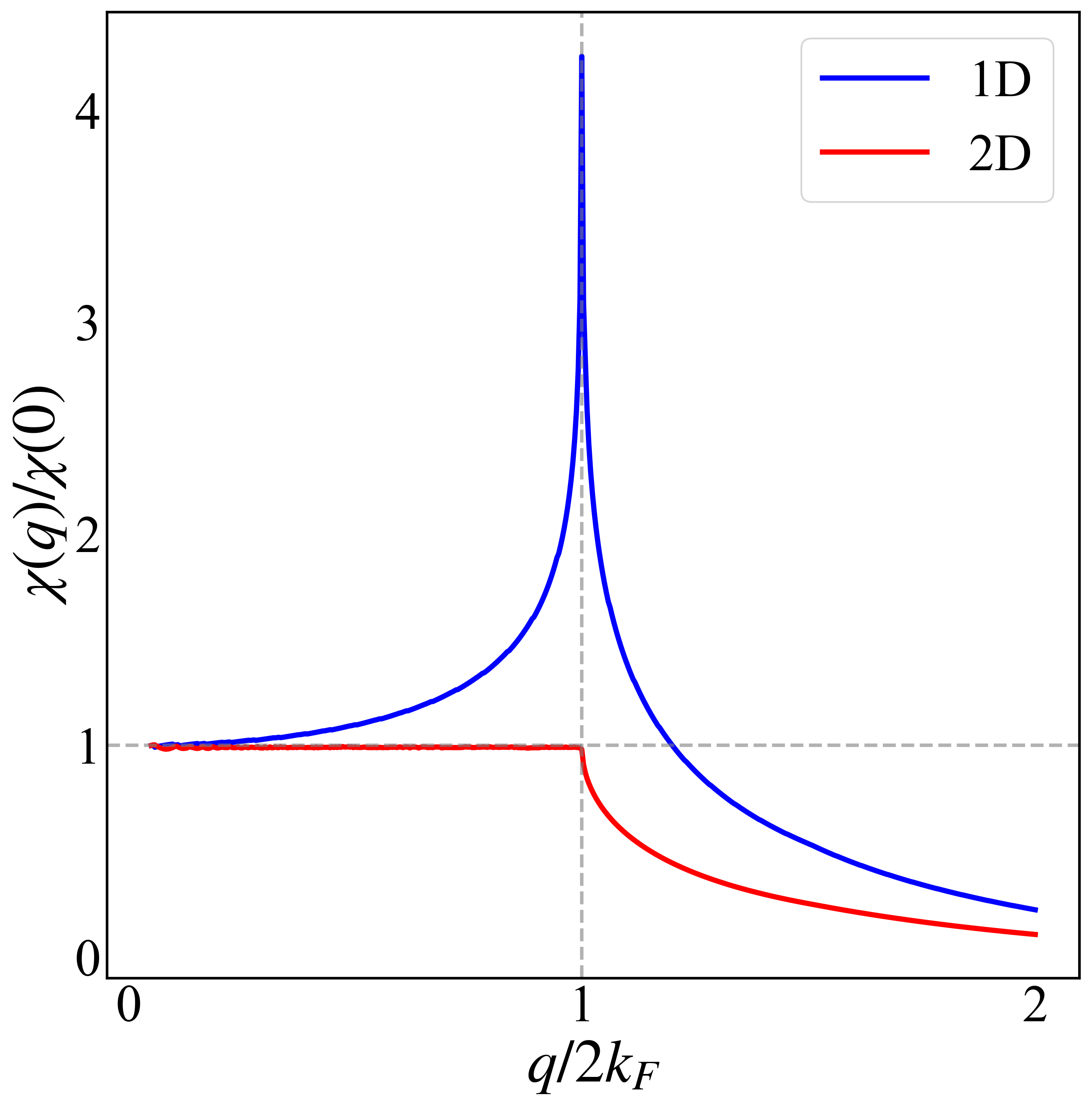
一维与二维体系的静态极化率(数值计算)
极化率计算公式为
这里对一维和二维自由电子模型计算极化率,使用连续模型进行计算, 目的是为了方便与解析上的分析对应。
- 计算程序
1 | using Distributed |
- 绘图程序
1
2
3
4
5
6
7
8
9
10
11
12
13
14
15
16
17
18
19
20
21
22
23
24
25
26
27
28
29
30
31
32
33
34
35
36
37
38
39
40
41
42
43
44
45
46
47
48
49
50
51
52
53
54
55
56
57
58
59
60
61
62
63
64
65
66
67
68
69
70
71
72
73
74
75
import numpy as np
import matplotlib.pyplot as plt
from matplotlib import rcParams
import os
# 1. Latex 字体与全局样式设置
plt.rc('font', family='Times New Roman')
config = {
"font.size": 22,
"mathtext.fontset": 'stix',
"axes.unicode_minus": False
}
rcParams.update(config)
#------------------------------------------------------------------------------------
def plot_polarization(dat_file):
"""
整合 plotfs 风格与极化率特有的图例、辅助线标记
"""
if not os.path.exists(dat_file):
print(f"Error: File '{dat_file}' not found.")
return
# 1. 加载数据
data = np.loadtxt(dat_file)
x0 = data[:, 0] / 2.0 # 归一化 q/2kF
pi_1d = data[:, 1]
pi_2d = data[:, 2]
# 2. 创建画布 (参照 plotfs 10x10 比例)
plt.figure(figsize=(10, 10))
# 3. 绘图:保留颜色对比与图例标签
plt.plot(x0, pi_1d, lw=3, c="b", label="1D")
plt.plot(x0, pi_2d, lw=3, c="r", label="2D")
# 4. 保留物理标记:q=2kF (即 x=1.0) 的辅助虚线
plt.axvline(x=1.0, color='gray', linestyle='--', lw=2, alpha=0.6)
# 5. 字体与字号设置 (参照 plotfs)
font2 = {'family': 'Times New Roman',
'weight': 'normal',
'size': 35,
}
plt.xlabel(r"$q/2k_F$", font2)
plt.ylabel(r"$\chi(q)/\chi(0)$", font2)
# 6. 保留图例 (参照 plotfs 注释掉的 legend 逻辑并启用)
# 使用 markerscale=2 保证图例线段足够明显
plt.legend(loc='best', prop={'family': 'Times New Roman', 'size': 30})
# 7. 刻度参数设置 (完全参照 plotfs)
plt.tick_params(direction='in', axis='x', width=0, length=10, labelsize=30)
plt.tick_params(direction='in', axis='y', width=0, length=10, labelsize=30)
# 8. 边框加粗 (完全参照 plotfs)
ax = plt.gca()
ax.spines["bottom"].set_linewidth(1.5)
ax.spines["left"].set_linewidth(1.5)
ax.spines["right"].set_linewidth(1.5)
ax.spines["top"].set_linewidth(1.5)
# 9. 限制坐标刻度数量 (这是你要求的关键修改方式)
ax.locator_params(axis='x', nbins=3)
ax.locator_params(axis='y', nbins=5)
# 3. 辅助线
ax.axhline(y=1.0, color='gray', linestyle='--', linewidth=2, alpha=0.6)
# 10. 保存
picname = os.path.splitext(dat_file)[0] + ".png"
plt.savefig(picname, dpi=300, bbox_inches='tight')
plt.close()
#---------------------------------------------------------------------
if __name__ == "__main__":
plot_polarization("lindhard_continuous.dat")
鉴于该网站分享的大都是学习笔记,作者水平有限,若发现有问题可以发邮件给我
- yxliphy@gmail.com
也非常欢迎喜欢分享的小伙伴投稿
本博客所有文章除特别声明外,均采用 CC BY-NC-SA 4.0 许可协议。转载请注明来源 Yu-Xuan's Blog!


相关推荐

2025-10-02
迭代方法自能计算
最近在学习输运方面的内容,这篇Blog主要就是整理如何通过迭代格林函数的方式来计算电极与导体耦合之后的自能。不得不说知乎是个学习的好地方,我这里的主要内容也都是在知乎上学习的,自己整理一下再加上...
2026-01-11
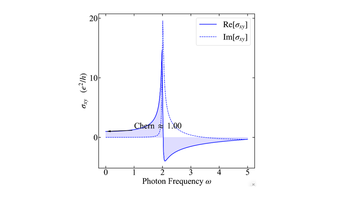
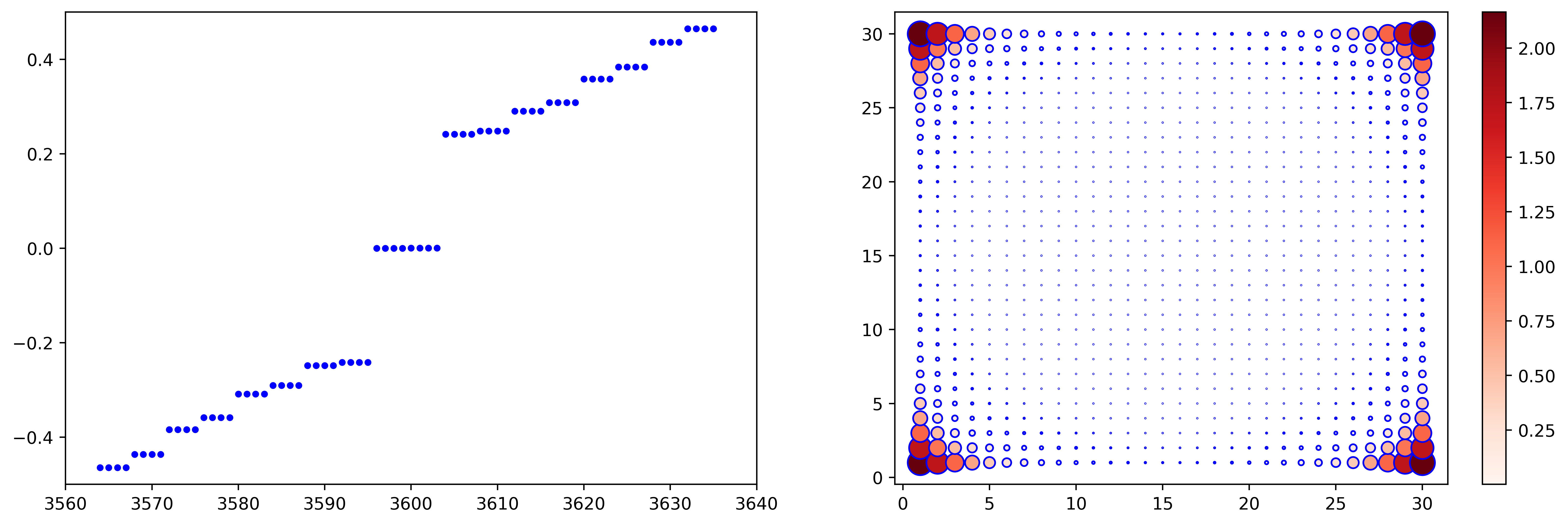
Hall电导以及光电导计算(Half-BHZ模型为例)
2019-04-17
Majorana Corner State in High Temperature Superconductor
最近刚刚学习了julia, 手头上也正好在重复一篇文章,就正好拿新学习的内容一边温习一边做研究。 导入函数库1234567# Import external package that use...
评论
公告

欢迎关注公众号,有趣的内容也会在上面同步。 有密码的文章属于正在建设中或者没有通过验证的内容,若有需要可通过邮件联系。