最近在看一本Berry Phase的书,上面的很多实例都是利用Pythtb这个有python写的包进行计算的,自己之前也接触过这个包,但是没有进一步学习,这里就把自己在学习这个包过程中一些自己的理解记录一下,这个内容还是会更新的,因为我觉得自己一遍并没有很好的对里面的内容完全理解.下面所有的内容都是官网上面的例子,我只是照抄过来运行,然后自己看代码理解一些参数以及函数的用途.
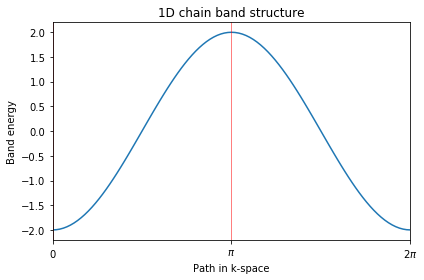
简单一维模型求解
#!/usr/bin/env python

# one dimension chain

from pythtb import * # 导入紧束缚类
import matplotlib.pyplot as plt # 导入作图包

# 定义模型
lat = [[1.0]]  # 元胞的基矢
orb = [[0.0]]  # 紧束缚模型中紧束缚轨道的位置,也就是要选择的原子轨道,其原子在元胞内的位置,它是会和元胞基矢相乘后计算的
my = tb_model(1,1,lat,orb)  # 1:k空间中是1维的   1: 实空间中是一维的
my.set_hop(-1,0,0,[1]) # 设置从0-->0 + 1 这个位置的hopping大小是 -1
(k_vec,k_dist,k_node)=my.k_path('full',100)  # 在全布里渊区中取100个点,knode是一些高对称点
k_label=[r"$0$",r"$\pi$", r"$2\pi$"]

evals=my.solve_all(k_vec) # 在由上面得到的布里渊区中的点上计算能带本征值

# plot band structure
fig, ax = plt.subplots()
ax.plot(k_dist,evals[0])
ax.set_title("1D chain band structure")
ax.set_xlabel("Path in k-space")
ax.set_ylabel("Band energy")
ax.set_xticks(k_node) # 将这些高对称点设置为坐标轴点
ax.set_xticklabels(k_label) # 设置坐标轴标签
ax.set_xlim(k_node[0],k_node[-1])  # 设置坐标轴范围
for n in range(len(k_node)):
    ax.axvline(x=k_node[n], linewidth=0.5, color='r')  # 通过循环得到高对称节点,在这些点上画竖线
fig.tight_layout()
fig.savefig("simple_band.pdf")
Path in 1D BZ defined by nodes at [0. 0.5 1. ]
二维模型求解
#!/usr/bin/env python
from __future__ import print_function
from pythtb import * # import TB model class
import numpy as np
import matplotlib.pyplot as plt
# define lattice vectors
lat=[[1.0,0.0],[0.0,1.0]] # 二维元胞的两个基矢,它们相互正交
# define coordinates of orbitals
orb=[[0.0,0.0],[0.5,0.5]] # 紧束缚轨道的位置,这里有两个轨道
# make two dimensional tight-binding checkerboard model
my_model = tb_model(2,2,lat,orb) # 定义自己的模型,k空间与实空间都是2维的
# set model parameters
delta = 1.1
t = 0.6
# set on-site energies
my_model.set_onsite([-delta,delta]) # 设置on-site上的能量,因为有两个轨道,所以这里赋值也是对两个轨道
# set hoppings (one for each connected pair of orbitals)
# (amplitude, i, j, [lattice vector to cell containing j])
my_model.set_hop(t, 1, 0, [0, 0]) # 第一个TB轨道到第二个TB轨道的hopping,R=[0,0],这是相当于在同一个cell内
my_model.set_hop(t, 1, 0, [1, 0]) # R=[1,0] 在x方向上不同元胞间的hopping
my_model.set_hop(t, 1, 0, [0, 1]) # R=[0,1] 在y方向上不同元胞间的hopping
my_model.set_hop(t, 1, 0, [1, 1]) # R = [1,1] 平移R之后,不同元胞间TB轨道上的hopping
# print tight-binding model
#my_model.display()
# generate k-point path and labels
path=[[0.0,0.0],[0.0,0.5],[0.5,0.5],[0.0,0.0]] # 自己定义一个2D BZ中的路径求解问题
label=(r'$\Gamma $',r'$X$', r'$M$', r'$\Gamma $') # 坐标轴标签要设置latex,需要使用r进行转义
(k_vec,k_dist,k_node)=my_model.k_path(path,301) # 在定义的路径上取点数为301个
print('---------------------------------------')
print('starting calculation')
print('---------------------------------------')
print('Calculating bands...')
# solve for eigenenergies of hamiltonian on
# the set of k-points from above
evals = my_model.solve_all(k_vec) # 在设置的路径上,对系统进行求解
# plotting of band structure
print('Plotting bandstructure...')
# First make a figure object
fig, ax = plt.subplots()
# specify horizontal axis details
ax.set_xlim(k_node[0],k_node[-1]) # 用求解得到的最大和最小值设置坐标轴范围
ax.set_xticks(k_node)
ax.set_xticklabels(label)
for n in range(len(k_node)):
ax.axvline(x=k_node[n], linewidth=0.5, color='r')
# plot bands
for n in range(2):
ax.plot(k_dist,evals[n]) # 能带图绘制
# put title
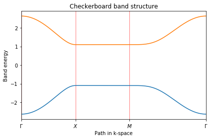
ax.set_title("Checkerboard band structure")
ax.set_xlabel("Path in k-space")
ax.set_ylabel("Band energy")
# make an PDF figure of a plot
fig.tight_layout() #
fig.savefig("checkerboard_band.pdf") # 将能带图保存成pdf文件
print('Done.\n')
----- k_path report begin ----------
real-space lattice vectors
 [[1. 0.]
 [0. 1.]]
k-space metric tensor
 [[1. 0.]
 [0. 1.]]
internal coordinates of nodes
 [[0.  0. ]
 [0.  0.5]
 [0.5 0.5]
 [0.  0. ]]
reciprocal-space lattice vectors
 [[1. 0.]
 [0. 1.]]
cartesian coordinates of nodes
 [[0.  0. ]
 [0.  0.5]
 [0.5 0.5]
 [0.  0. ]]
list of segments:
  length =     0.5  from  [0. 0.]  to  [0.  0.5]
  length =     0.5  from  [0.  0.5]  to  [0.5 0.5]
  length = 0.70711  from  [0.5 0.5]  to  [0. 0.]
node distance list: [0.      0.5     1.      1.70711]
node index list:    [  0  88 176 300]
----- k_path report end ------------

---------------------------------------
starting calculation
---------------------------------------
Calculating bands...
Plotting bandstructure...
Done.
#!/usr/bin/env python

from __future__ import print_function
from pythtb import * # import TB model class
import numpy as np
import matplotlib.pyplot as plt

# define lattice vectors
lat = [[2.0,0.0],[0.0,1.0]]  # 定义二维的元胞基矢
# define coordinates of orbitals
orb = [[0.0,0.0],[0.5,1.0]]  # 定义元胞中TB轨道的位置,也就是元胞中原子的位置,因为TB轨道也就是由这些原子贡献的

# make one dimensional tight-binding model of a trestle-like structure
my_model = tb_model(1,2,lat,orb,per=[0])  # k空间是1D,实空间是2D,半开边界的条件

# set model parameters
t_first = 0.8 + 0.6j
t_second = 2.0

# leave on-site energies to default zero values
# set hoppings (one for each connected pair of orbitals)
# (amplitude, i, j, [lattice vector to cell containing j])
my_model.set_hop(t_second, 0, 0, [1,0])  # 不同元胞之间第一个轨道间的hopping
my_model.set_hop(t_second, 1, 1, [1,0])  # 不同元胞之间第二个轨道间的hopping
my_model.set_hop(t_first, 0, 1, [0,0])   # 元胞内不同轨道间的hopping
my_model.set_hop(t_first, 1, 0, [1,0])   # 元胞间不同轨道间的hopping

# print tight-binding model
#my_model.display()  # Class内置的一个函数,用来查看自己构建的Hamiltonian模型

# generate list of k-points following some high-symmetry line in
(k_vec,k_dist,k_node) = my_model.k_path('fullc',100)   # 以Gamma点为中心的BZ
k_label = [r"$-\pi$",r"$0$", r"$\pi$"]

print('---------------------------------------')
print('starting calculation')
print('---------------------------------------')
print('Calculating bands...')

# solve for eigenenergies of hamiltonian on
# the set of k-points from above
evals = my_model.solve_all(k_vec)

# plotting of band structure
print('Plotting bandstructure...')

# First make a figure object
fig, ax = plt.subplots()
# specify horizontal axis details
ax.set_xlim(k_node[0],k_node[-1])
ax.set_xticks(k_node)
ax.set_xticklabels(k_label)
ax.axvline(x=k_node[1],linewidth=0.5, color='k')

# plot first band
ax.plot(k_dist,evals[0])
# plot second band
ax.plot(k_dist,evals[1])
# put title
ax.set_title("Trestle band structure")
ax.set_xlabel("Path in k-space")
ax.set_ylabel("Band energy")
# make an PDF figure of a plot
fig.tight_layout()
fig.savefig("trestle_band.pdf")

print('Done.\n')
 Path in 1D BZ defined by nodes at [-0.5  0.   0.5]

---------------------------------------
starting calculation
---------------------------------------
Calculating bands...
Plotting bandstructure...
Done.
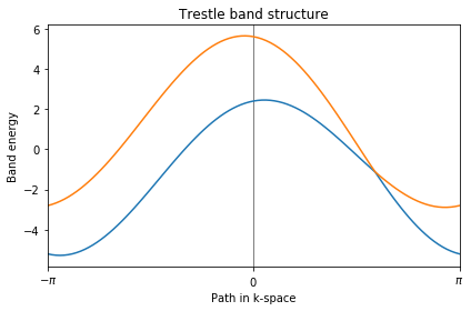
从能带的计算结果就可以看到,在构建模型的时候,每个元胞中是有两个轨道的,如果认为每个轨道来自不同的原子的话,也就是每个元胞中都是由2个原子的
#!/usr/bin/env python

# zero dimensional tight-binding model of a NH3 molecule

from __future__ import print_function
from pythtb import * # import TB model class
import numpy as np
import matplotlib.pyplot as plt

# define lattice vectors
lat=[[1.0,0.0,0.0],[0.0,1.0,0.0],[0.0,0.0,1.0]]  # 定义三维元胞基矢
# define coordinates of orbitals
sq32 = np.sqrt(3.0)/2.0
orb = [[ (2./3.)*sq32, 0.   ,0.],
     [(-1./3.)*sq32, 1./2.,0.],
     [(-1./3.)*sq32,-1./2.,0.],
     [  0.         , 0.   ,1.]]  # 一个氨气分子中由4个原子,假设每个原子贡献一个TB轨道,那么这里就会有4个轨道位置
# make zero dimensional tight-binding model
my_model = tb_model(0,3,lat,orb)  # 因为这里只有一个分子,所以不存在周期性,故k空间的维数就是0

# set model parameters
delta = 0.5
t_first = 1.0

# change on-site energies so that N and H don't have the same energy
my_model.set_onsite([-delta,-delta,-delta,delta])  # 对四个轨道分别设置on-site能量
# set hoppings (one for each connected pair of orbitals)
# (amplitude, i, j)
my_model.set_hop(t_first, 0, 1)  #  这里因为只有一个分子,所以也就不存在设置元胞平移矢量R
my_model.set_hop(t_first, 0, 2)
my_model.set_hop(t_first, 0, 3)
my_model.set_hop(t_first, 1, 2)
my_model.set_hop(t_first, 1, 3)
my_model.set_hop(t_first, 2, 3)

# print tight-binding model
#my_model.display()

print('---------------------------------------')
print('starting calculation')
print('---------------------------------------')
print('Calculating bands...')
print()
print('Band energies')
print()
# solve for eigenenergies of hamiltonian
evals = my_model.solve_all()   # 对于一个单分子体系,这里设置了4个轨道,所以最后的结果也就是4个轨道对应的能量

# First make a figure object
fig, ax = plt.subplots()
# plot all states
ax.plot(evals,"bo")
ax.set_xlim(-0.3,3.3)
ax.set_ylim(evals.min() - 0.5,evals.max() + 0.5)
# put title
ax.set_title("Molecule levels")
ax.set_xlabel("Orbital")
ax.set_ylabel("Energy")
# make an PDF figure of a plot
fig.tight_layout()
fig.savefig("0dim_spectrum.pdf")

print('Done.\n')
---------------------------------------
starting calculation
---------------------------------------
Calculating bands...

Band energies

Done.
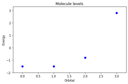
从计算结果也可以清楚的看到,一个分子中,也可以认为是一个元胞中有4个TB轨道,所以对于单分子进行求解之后,也就只有4个能量本征值
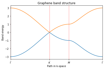
Graphene model
#!/usr/bin/env python

# Toy graphene model

from __future__ import print_function
from pythtb import * # import TB model class
import numpy as np
import matplotlib.pyplot as plt

# define lattice vectors
lat=[[1.0,0.0],[0.5,np.sqrt(3.0)/2.0]]  # 石墨烯的元胞基矢
# define coordinates of orbitals
orb=[[1./3.,1./3.],[2./3.,2./3.]]    # 石墨烯一个元胞中存在两个不等价的原子,也就是说贡献两个TB轨道

# make two dimensional tight-binding graphene model
my_model = tb_model(2,2,lat,orb)  # 实空间与k空间都是2维的

# set model parameters
delta = 0.0
t = -1.0

# set on-site energies
my_model.set_onsite([-delta,delta])  # 两个轨道on-site能量设置
# set hoppings (one for each connected pair of orbitals)
# (amplitude, i, j, [lattice vector to cell containing j])
my_model.set_hop(t, 0, 1, [ 0, 0])  # 元胞内TB轨道间的hopping
my_model.set_hop(t, 1, 0, [ 1, 0])  # 元胞间TB轨道间的hopping
my_model.set_hop(t, 1, 0, [ 0, 1])

# print tight-binding model
#my_model.display()

# generate list of k-points following a segmented path in the BZ
# list of nodes (high-symmetry points) that will be connected
path = [[0.,0.],[2./3.,1./3.],[.5,.5],[0.,0.]]  # k空间中进行求解的路径
# labels of the nodes
label=(r'$\Gamma $',r'$K$', r'$M$', r'$\Gamma $')
# total number of interpolated k-points along the path
nk = 121

# call function k_path to construct the actual path
(k_vec,k_dist,k_node) = my_model.k_path(path,nk)
# inputs:
#   path, nk: see above
#   my_model: the pythtb model
# outputs:
#   k_vec: list of interpolated k-points
#   k_dist: horizontal axis position of each k-point in the list
#   k_node: horizontal axis position of each original node

print('---------------------------------------')
print('starting calculation')
print('---------------------------------------')
print('Calculating bands...')

# obtain eigenvalues to be plotted
evals = my_model.solve_all(k_vec)  # 这里计算得到模型的本征值

# figure for bandstructure

fig, ax = plt.subplots()
# specify horizontal axis details
# set range of horizontal axis
ax.set_xlim(k_node[0],k_node[-1])
# put tickmarks and labels at node positions
ax.set_xticks(k_node)
ax.set_xticklabels(label)
# add vertical lines at node positions
for n in range(len(k_node)):
    ax.axvline(x=k_node[n],linewidth=0.5, color='r')
# put title
ax.set_title("Graphene band structure")
ax.set_xlabel("Path in k-space")
ax.set_ylabel("Band energy")

# plot first and second band
ax.plot(k_dist,evals[0])
ax.plot(k_dist,evals[1])

# make an PDF figure of a plot
fig.tight_layout()
fig.savefig("graphene.pdf")

print('Done.\n')
----- k_path report begin ----------
real-space lattice vectors
 [[1.      0.     ]
 [0.5     0.86603]]
k-space metric tensor
 [[ 1.33333 -0.66667]
 [-0.66667  1.33333]]
internal coordinates of nodes
 [[0.      0.     ]
 [0.66667 0.33333]
 [0.5     0.5    ]
 [0.      0.     ]]
reciprocal-space lattice vectors
 [[ 1.      -0.57735]
 [ 0.       1.1547 ]]
cartesian coordinates of nodes
 [[0.      0.     ]
 [0.66667 0.     ]
 [0.5     0.28868]
 [0.      0.     ]]
list of segments:
  length = 0.66667  from  [0. 0.]  to  [0.66667 0.33333]
  length = 0.33333  from  [0.66667 0.33333]  to  [0.5 0.5]
  length = 0.57735  from  [0.5 0.5]  to  [0. 0.]
node distance list: [0.      0.66667 1.      1.57735]
node index list:    [  0  51  76 120]
----- k_path report end ------------

---------------------------------------
starting calculation
---------------------------------------
Calculating bands...
Done.
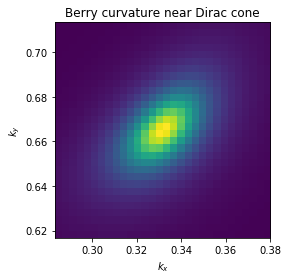
Berry phase around Dirac cone in graphene
#!/usr/bin/env python

# Compute Berry phase around Dirac cone in
# graphene with staggered onsite term delta

from __future__ import print_function
from pythtb import * # import TB model class
import numpy as np
import matplotlib.pyplot as plt

# define lattice vectors
lat = [[1.0,0.0],[0.5,np.sqrt(3.0)/2.0]]
# define coordinates of orbitals
orb = [[1./3.,1./3.],[2./3.,2./3.]]

# make two dimensional tight-binding graphene model
my_model = tb_model(2,2,lat,orb)

# set model parameters
delta = -0.1 # small staggered onsite term
t = -1.0

# set on-site energies
my_model.set_onsite([-delta,delta])
# set hoppings (one for each connected pair of orbitals)
# (amplitude, i, j, [lattice vector to cell containing j])
my_model.set_hop(t, 0, 1, [ 0, 0])
my_model.set_hop(t, 1, 0, [ 1, 0])
my_model.set_hop(t, 1, 0, [ 0, 1])

# print tight-binding model
#my_model.display()

# construct circular path around Dirac cone
#   parameters of the path
circ_step = 31
circ_center = np.array([1.0/3.0,2.0/3.0])
circ_radius = 0.05
# one-dimensional wf_array to store wavefunctions on the path
w_circ = wf_array(my_model,[circ_step])
# now populate array with wavefunctions
for i in range(circ_step):
    # construct k-point coordinate on the path
    ang = 2.0*np.pi*float(i)/float(circ_step-1)
    kpt = np.array([np.cos(ang)*circ_radius,np.sin(ang)*circ_radius])  # 以circ_center为中心的一个闭合路径
    kpt += circ_center
    # find eigenvectors at this k-point
    (eval,evec) = my_model.solve_one(kpt,eig_vectors = True)
    # store eigenvector into wf_array object
    w_circ[i] = evec
# make sure that first and last points are the same
w_circ[-1] = w_circ[0]  # 强制初末位置上的本征矢量是相同的,保证是一个完整的路径

# compute Berry phase along circular path

print("Berry phase along circle with radius: ",circ_radius)
print("  centered at k-point: ",circ_center)
print("  for band 0 equals    : ", w_circ.berry_phase([0],0))  # 计算第一个占据态的Berry位相,沿着0设置的这个方向
print("  for band 1 equals    : ", w_circ.berry_phase([1],0))
print("  for both bands equals: ", w_circ.berry_phase([0,1],0)) # 计算前两个占据态的Berry位相
print()

# construct two-dimensional square patch covering the Dirac cone
#  parameters of the patch
square_step = 31
square_center = np.array([1.0/3.0,2.0/3.0]) # 确定一个中心位置,在这个的基础上构建正方点阵计算Berry曲率
square_length = 0.1
# two-dimensional wf_array to store wavefunctions on the path
w_square = wf_array(my_model,[square_step,square_step]) # 构造正方形点阵,在其上计算波函数
all_kpt = np.zeros((square_step,square_step,2))
# now populate array with wavefunctions
for i in range(square_step):
    for j in range(square_step):
        # construct k-point on the square patch
        kpt = np.array([square_length*(-0.5 + float(i)/float(square_step - 1)),
                      square_length*(-0.5 + float(j)/float(square_step - 1))])
        kpt += square_center
        # store k-points for plotting
        all_kpt[i,j,:] = kpt
        # find eigenvectors at this k-point
        (eval,evec) = my_model.solve_one(kpt,eig_vectors=True) # 在确定的k点上求解模型
        # store eigenvector into wf_array object
        w_square[i,j] = evec

# compute Berry flux on this square patch
print("Berry flux on square patch with length: ",square_length)
print("  centered at k-point: ",square_center)
print("  for band 0 equals    : ", w_square.berry_flux([0]))
print("  for band 1 equals    : ", w_square.berry_flux([1]))
print("  for both bands equals: ", w_square.berry_flux([0,1]))
print()

# also plot Berry phase on each small plaquette of the mesh
plaq = w_square.berry_flux([0],individual_phases = True) # 对于第一个占据态计算Berry曲率
#
fig, ax = plt.subplots()
ax.imshow(plaq.T,origin="lower",
          extent=(all_kpt[0,0,0],all_kpt[-2, 0,0],
                  all_kpt[0,0,1],all_kpt[ 0,-2,1],))
ax.set_title("Berry curvature near Dirac cone")
ax.set_xlabel(r"$k_x$")
ax.set_ylabel(r"$k_y$")
fig.tight_layout()
fig.savefig("cone_phases.pdf")

print('Done.\n')
Berry phase along circle with radius:  0.05
  centered at k-point:  [0.33333333 0.66666667]
  for band 0 equals    :  2.068204018990522
  for band 1 equals    :  -2.068204018990522
  for both bands equals:  3.469446951953614e-17

Berry flux on square patch with length:  0.1
  centered at k-point:  [0.33333333 0.66666667]
  for band 0 equals    :  2.179216480131516
  for band 1 equals    :  -2.1792164801315166
  for both bands equals:  3.308776163370093e-16

Done.
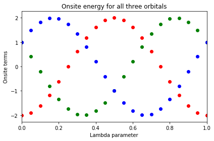
One-dimensional cycle of 1D tight-binding model
#!/usr/bin/env python
# one-dimensional family of tight binding models
# parametrized by one parameter, lambda
from __future__ import print_function
from pythtb import * # import TB model class
import numpy as np
import matplotlib.pyplot as plt
# define lattice vectors
lat = [[1.0]] # 1D元胞的基矢
# define coordinates of orbitals
orb = [[0.0],[1.0/3.0],[2.0/3.0]] # 每个元胞中有3个TB轨道,位置如设置所示,这个数值是要进行约化的
# make one dimensional tight-binding model
my_model = tb_model(1,1,lat,orb) # 构建TB模型
# set model parameters
delta = 2.0
t = -1.0
# set hoppings (one for each connected pair of orbitals)
# (amplitude, i, j, [lattice vector to cell containing j])
my_model.set_hop(t, 0, 1, [0]) # 元胞内第一个轨道向第二个轨道hopping
my_model.set_hop(t, 1, 2, [0]) # 元胞内第二个轨道向第三个轨道hopping
my_model.set_hop(t, 2, 0, [1]) # 元胞间第三个轨道向第一个轨道hopping
# plot onsite terms for each site
fig_onsite, ax_onsite = plt.subplots()
# plot band structure for each lambda
fig_band, ax_band = plt.subplots()
# evolve tight-binding parameter along some path by
# performing a change of onsite terms
# how many steps to take along the path (including end points)
path_steps = 21 # 控制参数撒点的数目
# create lambda mesh from 0.0 to 1.0 (21 values and 20 intervals)
all_lambda = np.linspace(0.0,1.0,path_steps,endpoint=True)
# how many k-points to use (31 values and 30 intervals)
num_kpt = 31 # 控制k点的数目
# two-dimensional wf_array in which we will store wavefunctions
# for all k-points and all values of lambda. (note that the index
# order [k,lambda] is important for interpreting the sign.)
wf_kpt_lambda = wf_array(my_model,[num_kpt,path_steps]) # 根据点数控制,构建一个参数空间
for i_lambda in range(path_steps):
# for each step along the path compute onsite terms for each orbital
lmbd = all_lambda[i_lambda]
onsite_0 = delta*(-1.0)*np.cos(2.0*np.pi*(lmbd - 0.0/3.0)) # 3个随着循环变化的量,在后面作为元胞内TB轨道的on-site能量
onsite_1 = delta*(-1.0)*np.cos(2.0*np.pi*(lmbd - 1.0/3.0))
onsite_2 = delta*(-1.0)*np.cos(2.0*np.pi*(lmbd - 2.0/3.0))
# update onsite terms by rewriting previous values
my_model.set_onsite([onsite_0,onsite_1,onsite_2],mode="reset")
# create k mesh over 1D Brillouin zone
(k_vec,k_dist,k_node) = my_model.k_path([[-0.5],[0.5]],num_kpt,report=False)
# solve model on all of these k-points
(eval,evec) = my_model.solve_all(k_vec,eig_vectors=True)
# store wavefunctions (eigenvectors)
for i_kpt in range(num_kpt):
wf_kpt_lambda[i_kpt,i_lambda] = evec[:,i_kpt,:] # 将计算得到的波函数单独存储
# plot on-site terms
# 在这里绘制三个on-site能量的变化曲线
ax_onsite.scatter([lmbd],[onsite_0],c = "r")
ax_onsite.scatter([lmbd],[onsite_1],c = "g")
ax_onsite.scatter([lmbd],[onsite_2],c = "b")
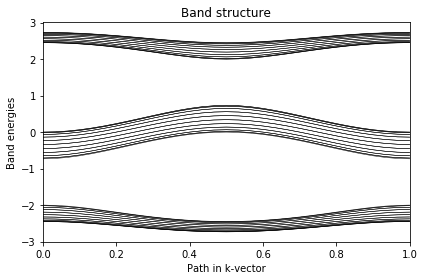
# plot band structure for all three bands
for band in range(eval.shape[0]):
ax_band.plot(k_dist,eval[band,:],"k-",linewidth=0.5)
# impose periodic boundary condition along k-space direction only
# (so that |psi_nk> at k=0 and k=1 have the same phase)
# 将参数演化空间中,首尾的波函数强制相等起来
wf_kpt_lambda.impose_pbc(0,0)
# compute Berry phase along k-direction for each lambda
phase = wf_kpt_lambda.berry_phase([0],0) # 计算第一个占据态沿着参数演化的Berry位相
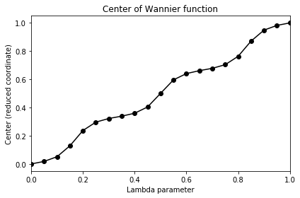
# plot position of Wannier function for bottom band
fig_wann, ax_wann = plt.subplots()
# wannier center in reduced coordinates
wann_center = phase/(2.0*np.pi)
# plot wannier centers
ax_wann.plot(all_lambda,wann_center,"ko-")
# compute integrated curvature
final = wf_kpt_lambda.berry_flux([0]) # 在这个参数空间中计算Berry曲率
print("Berry flux in k-lambda space: ",final)
# finish plot of onsite terms
ax_onsite.set_title("Onsite energy for all three orbitals")
ax_onsite.set_xlabel("Lambda parameter")
ax_onsite.set_ylabel("Onsite terms")
ax_onsite.set_xlim(0.0,1.0)
fig_onsite.tight_layout()
fig_onsite.savefig("3site_onsite.pdf")
# finish plot for band structure
ax_band.set_title("Band structure")
ax_band.set_xlabel("Path in k-vector")
ax_band.set_ylabel("Band energies")
ax_band.set_xlim(0.0,1.0)
fig_band.tight_layout()
fig_band.savefig("3site_band.pdf")
# finish plot for Wannier center
ax_wann.set_title("Center of Wannier function")
ax_wann.set_xlabel("Lambda parameter")
ax_wann.set_ylabel("Center (reduced coordinate)")
ax_wann.set_xlim(0.0,1.0)
fig_wann.tight_layout()
fig_wann.savefig("3site_wann.pdf")
print('Done.\n')
Berry flux in k-lambda space:  -6.283185307179586
Done.
One-dimensional cycle on a finite 1D chain
#!/usr/bin/env python
# one-dimensional family of tight binding models
# parametrized by one parameter, lambda
from __future__ import print_function
from pythtb import * # import TB model class
import numpy as np
import matplotlib.pyplot as plt
# define function to construct model
def set_model(t,delta,lmbd):
lat = [[1.0]] # 1D元胞基矢
orb = [[0.0],[1.0/3.0],[2.0/3.0]] # 每个元胞中有三个轨道
model = tb_model(1,1,lat,orb) # 实空间与k空间都是1维的
model.set_hop(t, 0, 1, [0])
model.set_hop(t, 1, 2, [0])
model.set_hop(t, 2, 0, [1])
onsite_0 = delta*(-1.0)*np.cos(2.0*np.pi*(lmbd - 0.0/3.0))
onsite_1 = delta*(-1.0)*np.cos(2.0*np.pi*(lmbd - 1.0/3.0))
onsite_2 = delta*(-1.0)*np.cos(2.0*np.pi*(lmbd - 2.0/3.0))
model.set_onsite([onsite_0,onsite_1,onsite_2]) # 对每个轨道的on-site能进行设置,每个元胞中有三个轨道,则此处就设置三个值
return(model) # 最后返回一个构建好的模型
# set model parameters
delta = 2.0
t = -1.3
# evolve tight-binding parameter lambda along a path
path_steps = 21 # 设置演化参数的取点数
all_lambda = np.linspace(0.0,1.0,path_steps,endpoint=True) # 选取演化参数变化范围
# get model at arbitrary lambda for initializations
my_model = set_model(t,delta,0.) # 通过重新改写的函数定义模型
# set up 1d Brillouin zone mesh
num_kpt = 31 # 控制BZ中的去点数
(k_vec,k_dist,k_node) = my_model.k_path([[-0.5],[0.5]],num_kpt,report=False) # 设置BZ中进行计算的路径
# two-dimensional wf_array in which we will store wavefunctions
# we store it in the order [lambda,k] since want Berry curvatures
# and Chern numbers defined with the [lambda,k] sign convention
wf_kpt_lambda = wf_array(my_model,[path_steps,num_kpt])# 对模型,在参数空间构建一系列的点,这个由第二个参数来控制
# fill the array with eigensolutions
for i_lambda in range(path_steps):
lmbd = all_lambda[i_lambda] #循环索引参数点
my_model = set_model(t,delta,lmbd) # 在索引的参数下构建模型
(eval,evec) = my_model.solve_all(k_vec,eig_vectors=True) # 对模型进行求解
for i_kpt in range(num_kpt):
wf_kpt_lambda[i_lambda,i_kpt] = evec[:,i_kpt,:] # 把求解出来的波函数重新赋值给前面构建出来的数组
# compute integrated curvature
print("Chern numbers for rising fillings")
print(" Band 0 = %5.2f" % (wf_kpt_lambda.berry_flux([0])/(2.*np.pi))) # 计算第一个能带的Berry曲率
print(" Bands 0,1 = %5.2f" % (wf_kpt_lambda.berry_flux([0,1])/(2.*np.pi)))# 计算前两个能带
print(" Bands 0,1,2 = %5.2f" % (wf_kpt_lambda.berry_flux([0,1,2])/(2.*np.pi))) # 计算三个能带的结果之和
print("")
print("Chern numbers for individual bands")
print(" Band 0 = %5.2f" % (wf_kpt_lambda.berry_flux([0])/(2.*np.pi))) # 分别计算不同能带的Berry曲率
print(" Band 1 = %5.2f" % (wf_kpt_lambda.berry_flux([1])/(2.*np.pi)))
print(" Band 2 = %5.2f" % (wf_kpt_lambda.berry_flux([2])/(2.*np.pi)))
print("")
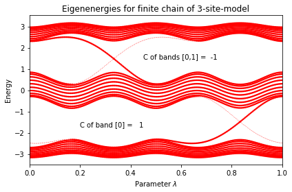
# for annotating plot with text
text_lower = "C of band [0] = %3.0f" % (wf_kpt_lambda.berry_flux([0])/(2.*np.pi))
text_upper = "C of bands [0,1] = %3.0f" % (wf_kpt_lambda.berry_flux([0,1])/(2.*np.pi))
# now loop over parameter again, this time for finite chains
path_steps = 241 # 重新构建一个参数空间,这个参数用来控制参数演化的取点数目
all_lambda = np.linspace(0.0,1.0,path_steps,endpoint=True) # 构建参数演化
# length of chain, in unit cells
num_cells = 10 # 取10个元胞
num_orb = 3*num_cells # 每个元胞有3个轨道,所以这是就共有30个轨道
# initialize array for chain eigenvalues and x expectations
ch_eval = np.zeros([num_orb,path_steps],dtype=float)
ch_xexp = np.zeros([num_orb,path_steps],dtype=float)
for i_lambda in range(path_steps):
lmbd = all_lambda[i_lambda] # 索引演化参数
# construct and solve model
my_model = set_model(t,delta,lmbd)
ch_model = my_model.cut_piece(num_cells,0) # 构建在一个方向上周期的结构,第一个参数控制重复的元胞数目,第二个参数决定选取哪个方向是周期的
(eval,evec) = ch_model.solve_all(eig_vectors=True) # 对重新构建好的模型进行计算
# save eigenvalues
ch_eval[:,i_lambda] = eval
ch_xexp[:,i_lambda] = ch_model.position_expectation(evec,0) # 求解位置算符的对角本征元,第一个参数是求解得到的本征矢,第二个参数控制计算哪个方向
# plot eigenvalues vs. lambda
# symbol size is reduced for states localized near left end
(fig, ax) = plt.subplots()
# loop over "bands"
for n in range(num_orb):
# diminish the size of the ones on the borderline
xcut = 2. # discard points below this
xfull = 4. # use sybols of full size above this
size = (ch_xexp[n,:] - xcut)/(xfull - xcut)
for i in range(path_steps):
size[i] = min(size[i],1.)
size[i] = max(size[i],0.1)
ax.scatter(all_lambda[:],ch_eval[n,:], edgecolors='none', s=size*6., c='r')
# annotate gaps with bulk Chern numbers calculated earlier
ax.text(0.20,-1.7,text_lower)
ax.text(0.45, 1.5,text_upper)
ax.set_title("Eigenenergies for finite chain of 3-site-model")
ax.set_xlabel(r"Parameter $\lambda$")
ax.set_ylabel("Energy")
ax.set_xlim(0.,1.)
fig.tight_layout()
fig.savefig("3site_endstates.pdf")
print('Done.\n')
Chern numbers for rising fillings
  Band  0     =  1.00
  Bands 0,1   = -1.00
  Bands 0,1,2 = -0.00

Chern numbers for individual bands
  Band  0 =  1.00
  Band  1 = -2.00
  Band  2 =  1.00

Done.
Haldane model
#!/usr/bin/env python
# Haldane model from Phys. Rev. Lett. 61, 2015 (1988)
from __future__ import print_function
from pythtb import * # import TB model class
import numpy as np
import matplotlib.pyplot as plt
# define lattice vectors
lat = [[1.0,0.0],[0.5,np.sqrt(3.0)/2.0]] # Graphene元胞基矢
# define coordinates of orbitals
orb = [[1./3.,1./3.],[2./3.,2./3.]] # 元胞中有两个原子,也就是说有两个轨道
# make two dimensional tight-binding Haldane model
my_model = tb_model(2,2,lat,orb) # 实空间与k空间都是两维的
# set model parameters
delta = 0.2
t = -1.0
t2 = 0.15*np.exp((1.j)*np.pi/2.)
t2c = t2.conjugate()
# set on-site energies
my_model.set_onsite([-delta,delta]) # 设置每个轨道on-site能量
# set hoppings (one for each connected pair of orbitals)
# (amplitude, i, j, [lattice vector to cell containing j])
my_model.set_hop(t, 0, 1, [ 0, 0]) # 元胞内轨道间的hopping设置
my_model.set_hop(t, 1, 0, [ 1, 0]) # 元胞间不同轨道之间的hopping
my_model.set_hop(t, 1, 0, [ 0, 1])
# add second neighbour complex hoppings
my_model.set_hop(t2 , 0, 0, [ 1, 0]) # Graphene次近邻都是在相同的轨道间的hopping,只不过是在不同的元胞之间,一共有6个次近邻
my_model.set_hop(t2 , 1, 1, [ 1,-1])
my_model.set_hop(t2 , 1, 1, [ 0, 1])
my_model.set_hop(t2c, 1, 1, [ 1, 0])
my_model.set_hop(t2c, 0, 0, [ 1,-1])
my_model.set_hop(t2c, 0, 0, [ 0, 1])
# print tight-binding model
#my_model.display()
# generate list of k-points following a segmented path in the BZ
# list of nodes (high-symmetry points) that will be connected
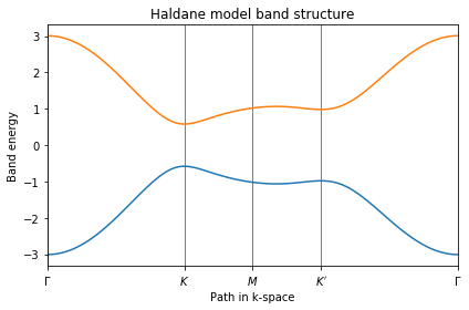
path = [[0.,0.],[2./3.,1./3.],[.5,.5],[1./3.,2./3.], [0.,0.]] # BZ中计算路径
# labels of the nodes
label = (r'$\Gamma $',r'$K$', r'$M$', r'$K^\prime$', r'$\Gamma $')
# call function k_path to construct the actual path
(k_vec,k_dist,k_node) = my_model.k_path(path,101) # 设置需要求解的路径,第二个参数控制撒点数
# inputs:
# path: see above
# 101: number of interpolated k-points to be plotted
# outputs:
# k_vec: list of interpolated k-points
# k_dist: horizontal axis position of each k-point in the list
# k_node: horizontal axis position of each original node
# obtain eigenvalues to be plotted
evals = my_model.solve_all(k_vec) # 求解模型在路径上的本征值
# figure for bandstructure
fig, ax = plt.subplots()
# specify horizontal axis details
# set range of horizontal axis
ax.set_xlim(k_node[0],k_node[-1])
# put tickmarks and labels at node positions
ax.set_xticks(k_node)
ax.set_xticklabels(label)
# add vertical lines at node positions
for n in range(len(k_node)):
ax.axvline(x=k_node[n],linewidth=0.5, color='k')
# put title
ax.set_title("Haldane model band structure")
ax.set_xlabel("Path in k-space")
ax.set_ylabel("Band energy")
# plot first band
ax.plot(k_dist,evals[0])
# plot second band
ax.plot(k_dist,evals[1])
# make an PDF figure of a plot
fig.tight_layout()
fig.savefig("haldane_band.pdf")
print()
print('---------------------------------------')
print('starting DOS calculation')
print('---------------------------------------')
print('Calculating DOS...')
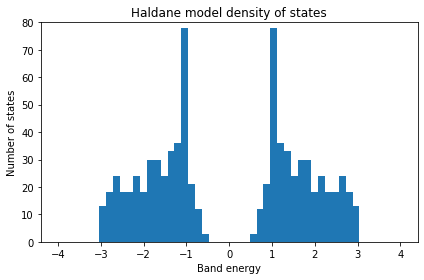
# calculate density of states
# first solve the model on a mesh and return all energies
kmesh = 20
kpts = []
for i in range(kmesh):
for j in range(kmesh):
kpts.append([float(i)/float(kmesh),float(j)/float(kmesh)]) # 构建一个点阵
# solve the model on this mesh
evals = my_model.solve_all(kpts) # 在所有的点阵点上求解本征值,某些点上的本征值可能相同,那么就说明这个能量下的态密度比较大
# flatten completely the matrix
evals = evals.flatten()
# plotting DOS
print('Plotting DOS...')
# now plot density of states
fig, ax = plt.subplots()
ax.hist(evals,50,range=(-4.,4.))
ax.set_ylim(0.0,80.0)
# put title
ax.set_title("Haldane model density of states")
ax.set_xlabel("Band energy")
ax.set_ylabel("Number of states")
# make an PDF figure of a plot
fig.tight_layout()
fig.savefig("haldane_dos.pdf")
print('Done.\n')
----- k_path report begin ----------
real-space lattice vectors
 [[1.      0.     ]
 [0.5     0.86603]]
k-space metric tensor
 [[ 1.33333 -0.66667]
 [-0.66667  1.33333]]
internal coordinates of nodes
 [[0.      0.     ]
 [0.66667 0.33333]
 [0.5     0.5    ]
 [0.33333 0.66667]
 [0.      0.     ]]
reciprocal-space lattice vectors
 [[ 1.      -0.57735]
 [ 0.       1.1547 ]]
cartesian coordinates of nodes
 [[0.      0.     ]
 [0.66667 0.     ]
 [0.5     0.28868]
 [0.33333 0.57735]
 [0.      0.     ]]
list of segments:
  length = 0.66667  from  [0. 0.]  to  [0.66667 0.33333]
  length = 0.33333  from  [0.66667 0.33333]  to  [0.5 0.5]
  length = 0.33333  from  [0.5 0.5]  to  [0.33333 0.66667]
  length = 0.66667  from  [0.33333 0.66667]  to  [0. 0.]
node distance list: [0.      0.66667 1.      1.33333 2.     ]
node index list:    [  0  33  50  67 100]
----- k_path report end ------------


---------------------------------------
starting DOS calculation
---------------------------------------
Calculating DOS...
Plotting DOS...
Done.
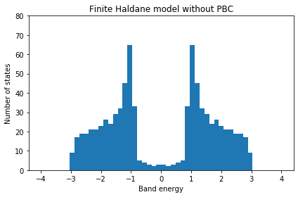
Finite Haldane model
#!/usr/bin/env python

# Haldane model from Phys. Rev. Lett. 61, 2015 (1988)
# Calculates density of states for finite sample of Haldane model

from __future__ import print_function
from pythtb import * # import TB model class
import numpy as np
import matplotlib.pyplot as plt

# define lattice vectors
lat = [[1.0,0.0],[0.5,np.sqrt(3.0)/2.0]]
# define coordinates of orbitals
orb = [[1./3.,1./3.],[2./3.,2./3.]]

# make two dimensional tight-binding Haldane model
my_model = tb_model(2,2,lat,orb)

# set model parameters
delta = 0.0
t = -1.0
t2 = 0.15*np.exp((1.j)*np.pi/2.)
t2c = t2.conjugate()

# set on-site energies
my_model.set_onsite([-delta,delta])
# set hoppings (one for each connected pair of orbitals)
# (amplitude, i, j, [lattice vector to cell containing j])
my_model.set_hop(t, 0, 1, [ 0, 0])
my_model.set_hop(t, 1, 0, [ 1, 0])
my_model.set_hop(t, 1, 0, [ 0, 1])
# add second neighbour complex hoppings
my_model.set_hop(t2 , 0, 0, [ 1, 0])
my_model.set_hop(t2 , 1, 1, [ 1,-1])
my_model.set_hop(t2 , 1, 1, [ 0, 1])
my_model.set_hop(t2c, 1, 1, [ 1, 0])
my_model.set_hop(t2c, 0, 0, [ 1,-1])
my_model.set_hop(t2c, 0, 0, [ 0, 1])

# print tight-binding model details
#my_model.display()

# cutout finite model first along direction x with no PBC
tmp_model = my_model.cut_piece(20,0,glue_edgs = False)  # 构建一个重复20次cell的结构,并且不允许首尾端存在hopping,这是x方向
# cutout also along y direction
fin_model_false = tmp_model.cut_piece(20,1,glue_edgs = False)# 这是在y方向进行同样的操作方式

# cutout finite model first along direction x with PBC
tmp_model = my_model.cut_piece(20,0,glue_edgs = True)# 构建一个重复20次cell的结构,允许首尾端存在hopping,相当于还是一个周期结构
# cutout also along y direction
fin_model_true = tmp_model.cut_piece(20,1,glue_edgs = True)

# solve finite model
evals_false = fin_model_false.solve_all()
evals_false = evals_false.flatten()
evals_true = fin_model_true.solve_all()
evals_true = evals_true.flatten()

# now plot density of states
fig, ax = plt.subplots()
ax.hist(evals_false,50,range=(-4.,4.))
ax.set_ylim(0.0,80.0)
ax.set_title("Finite Haldane model without PBC")
ax.set_xlabel("Band energy")
ax.set_ylabel("Number of states")
fig.tight_layout()
fig.savefig("haldane_fin_dos_false.pdf")
fig, ax = plt.subplots()
ax.hist(evals_true,50,range=(-4.,4.))
ax.set_ylim(0.0,80.0)
ax.set_title("Finite Haldane model with PBC")
ax.set_xlabel("Band energy")
ax.set_ylabel("Number of states")
fig.tight_layout()
fig.savefig("haldane_fin_dos_true.pdf")

print('Done.\n')
Done.

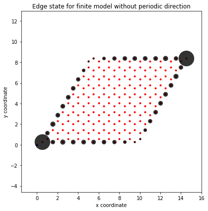
Edge states
#!/usr/bin/env python
# Haldane model from Phys. Rev. Lett. 61, 2015 (1988)
# Solves model and draws one of its edge states.
from __future__ import print_function
from pythtb import * # import TB model class
import numpy as np
# define lattice vectors
lat = [[1.0,0.0],[0.5,np.sqrt(3.0)/2.0]]
# define coordinates of orbitals
orb = [[1./3.,1./3.],[2./3.,2./3.]]
# make two dimensional tight-binding Haldane model
my_model = tb_model(2,2,lat,orb)
# set model parameters
delta = 0.0
t = -1.0
t2 = 0.15*np.exp((1.j)*np.pi/2.)
t2c = t2.conjugate()
# set on-site energies
my_model.set_onsite([-delta,delta])
# set hoppings (one for each connected pair of orbitals)
# (amplitude, i, j, [lattice vector to cell containing j])
my_model.set_hop(t, 0, 1, [ 0, 0])
my_model.set_hop(t, 1, 0, [ 1, 0])
my_model.set_hop(t, 1, 0, [ 0, 1])
# add second neighbour complex hoppings
my_model.set_hop(t2 , 0, 0, [ 1, 0])
my_model.set_hop(t2 , 1, 1, [ 1,-1])
my_model.set_hop(t2 , 1, 1, [ 0, 1])
my_model.set_hop(t2c, 1, 1, [ 1, 0])
my_model.set_hop(t2c, 0, 0, [ 1,-1])
my_model.set_hop(t2c, 0, 0, [ 0, 1])
# print tight-binding model details
#my_model.display()
# cutout finite model first along direction x with no PBC
tmp_model = my_model.cut_piece(10,0,glue_edgs=False) # x方向开边界取10个元胞
# cutout also along y direction with no PBC
fin_model = tmp_model.cut_piece(10,1,glue_edgs=False) # y方向取开边界取10个元胞
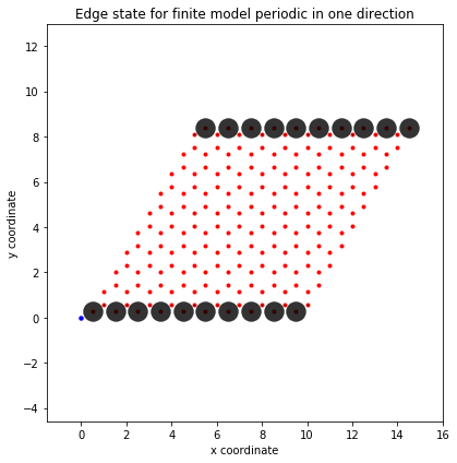
# cutout finite model first along direction x with PBC
tmp_model_half = my_model.cut_piece(10,0,glue_edgs = True) # 在x方向取10个元胞,然后首尾相连构成周期结构,相当于是半开边界情况
# cutout also along y direction with no PBC
fin_model_half = tmp_model_half.cut_piece(10,1,glue_edgs = False) # 在y方向取10个元胞,然后首尾相连构成周期结构
# solve finite models
(evals,evecs) = fin_model.solve_all(eig_vectors = True)
(evals_half,evecs_half) = fin_model_half.solve_all(eig_vectors = True)
# pick index of state in the middle of the gap
ed = fin_model.get_num_orbitals()//2 # 计算模型中有几个轨道
# draw one of the edge states in both cases
(fig,ax) = fin_model.visualize(0,1,eig_dr=evecs[ed,:],draw_hoppings=False) # 对模型进行可视化计算
ax.set_title("Edge state for finite model without periodic direction")
ax.set_xlabel("x coordinate")
ax.set_ylabel("y coordinate")
fig.tight_layout()
fig.savefig("edge_state.pdf")
#
(fig,ax)=fin_model_half.visualize(0,1,eig_dr=evecs_half[ed,:],draw_hoppings=False)
ax.set_title("Edge state for finite model periodic in one direction")
ax.set_xlabel("x coordinate")
ax.set_ylabel("y coordinate")
fig.tight_layout()
fig.savefig("edge_state_half.pdf")
print('Done.\n')
Done.
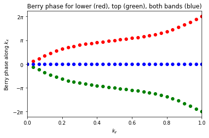
Berry phases in Haldane model
#!/usr/bin/env python

# Haldane model from Phys. Rev. Lett. 61, 2015 (1988)
# Calculates Berry phases and curvatures for this model

# Copyright under GNU General Public License 2010, 2012, 2016
# by Sinisa Coh and David Vanderbilt (see gpl-pythtb.txt)

from __future__ import print_function
from pythtb import * # import TB model class
import numpy as np
import matplotlib.pyplot as plt

# define lattice vectors
lat = [[1.0,0.0],[0.5,np.sqrt(3.0)/2.0]]
# define coordinates of orbitals
orb = [[1./3.,1./3.],[2./3.,2./3.]]

# make two dimensional tight-binding Haldane model
my_model = tb_model(2,2,lat,orb)

# set model parameters
delta=0.0
t=-1.0
t2 =0.15*np.exp((1.j)*np.pi/2.)
t2c=t2.conjugate()

# set on-site energies
my_model.set_onsite([-delta,delta])
# set hoppings (one for each connected pair of orbitals)
# (amplitude, i, j, [lattice vector to cell containing j])
my_model.set_hop(t, 0, 1, [ 0, 0])
my_model.set_hop(t, 1, 0, [ 1, 0])
my_model.set_hop(t, 1, 0, [ 0, 1])
# add second neighbour complex hoppings
my_model.set_hop(t2 , 0, 0, [ 1, 0])
my_model.set_hop(t2 , 1, 1, [ 1,-1])
my_model.set_hop(t2 , 1, 1, [ 0, 1])
my_model.set_hop(t2c, 1, 1, [ 1, 0])
my_model.set_hop(t2c, 0, 0, [ 1,-1])
my_model.set_hop(t2c, 0, 0, [ 0, 1])

# print tight-binding model details
#my_model.display()

print(r"Using approach #1")
# approach #1
# generate object of type wf_array that will be used for
# Berry phase and curvature calculations
my_array_1 = wf_array(my_model,[31,31])  # 构建计算Berry位相的点阵
# solve model on a regular grid, and put origin of
# Brillouin zone at -1/2 -1/2 point
my_array_1.solve_on_grid([-0.5,-0.5])  # 在给定的路径上计算

# calculate Berry phases around the BZ in the k_x direction
# (which can be interpreted as the 1D hybrid Wannier center
# in the x direction) and plot results as a function of k_y
#
# Berry phases along k_x for lower band
phi_a_1 = my_array_1.berry_phase([0],0,contin=True) # 计算第一个占据态的Berry位相
# Berry phases along k_x for upper band
phi_b_1 = my_array_1.berry_phase([1],0,contin=True) # 计算第二个占据态的Berry位相
# Berry phases along k_x for both bands
phi_c_1 = my_array_1.berry_phase([0,1],0,contin=True) # 计算前两个占据态的Berry位相

# Berry flux for lower band
flux_a_1 = my_array_1.berry_flux([0]) # 在k点阵上计算Berry曲率

# plot Berry phases
fig, ax = plt.subplots()
ky = np.linspace(0.,1.,len(phi_a_1))
ax.plot(ky,phi_a_1, 'ro')
ax.plot(ky,phi_b_1, 'go')
ax.plot(ky,phi_c_1, 'bo')
ax.set_title("Berry phase for lower (red), top (green), both bands (blue)")
ax.set_xlabel(r"$k_y$")
ax.set_ylabel(r"Berry phase along $k_x$")
ax.set_xlim(0.,1.)
ax.set_ylim(-7.,7.)
ax.yaxis.set_ticks([-2.*np.pi,-np.pi,0.,np.pi,2.*np.pi])
ax.set_yticklabels((r'$-2\pi$',r'$-\pi$',r'$0$',r'$\pi$', r'$2\pi$'))
fig.tight_layout()
fig.savefig("haldane_bp_phase.pdf")
# print out info about flux
print(" Berry flux= ",flux_a_1)

print(r"Using approach #2")
# approach #2
# do the same thing as in approach #1 but do not use
# automated solver
#
# intialize k-space mesh
nkx = 31  # 定义动量空间中的撒点数目
nky = 31
kx = np.linspace(-0.5,0.5,num=nkx)
ky = np.linspace(-0.5,0.5,num=nky)
# initialize object to store all wavefunctions
my_array_2 = wf_array(my_model,[nkx,nky])
# solve model at all k-points
for i in range(nkx):
    for j in range(nky):
        (eval,evec) = my_model.solve_one([kx[i],ky[j]],eig_vectors=True)  # 在每个点上对模型进行求解
        # store wavefunctions
        my_array_2[i,j] = evec
# impose periodic boundary conditions in both k_x and k_y directions
my_array_2.impose_pbc(0,0)
my_array_2.impose_pbc(1,1)
# calculate Berry flux for lower band
flux_a_2 = my_array_2.berry_flux([0])

# print out info about curvature
print(" Berry flux= ",flux_a_2)

print('Done.\n')
Using approach #1
 Berry flux=  -6.283185307179586
Using approach #2
 Berry flux=  -6.283185307179586
Done.
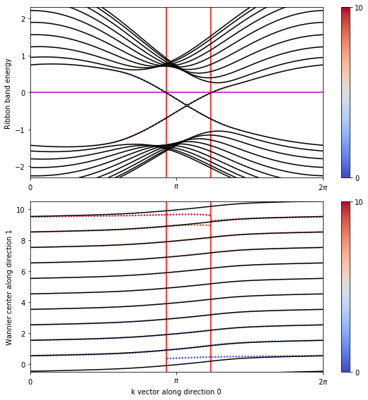
Hybrid Wannier centers in Haldane model
#!/usr/bin/env python

# Haldane model from Phys. Rev. Lett. 61, 2015 (1988)
# First, compute bulk Wannier centers along direction 1
# Then, cut a ribbon that extends along direcion 0, and compute
#   both the edge states and the finite hybrid Wannier centers
#   along direction 1.

from __future__ import print_function
from pythtb import * # import TB model class
import numpy as np
import matplotlib.pyplot as plt

# set model parameters
delta = -0.2
t = -1.0
t2 = 0.05-0.15j
t2c = t2.conjugate()

# Fermi level, relevant for edge states of ribbon
efermi = 0.25

# define lattice vectors and orbitals and make model
lat = [[1.0,0.0],[0.5,np.sqrt(3.0)/2.0]]
orb = [[1./3.,1./3.],[2./3.,2./3.]]
my_model = tb_model(2,2,lat,orb)

# set on-site energies and hoppings
my_model.set_onsite([-delta,delta])
my_model.set_hop(t, 0, 1, [ 0, 0])
my_model.set_hop(t, 1, 0, [ 1, 0])
my_model.set_hop(t, 1, 0, [ 0, 1])
my_model.set_hop(t2 , 0, 0, [ 1, 0])
my_model.set_hop(t2 , 1, 1, [ 1,-1])
my_model.set_hop(t2 , 1, 1, [ 0, 1])
my_model.set_hop(t2c, 1, 1, [ 1, 0])
my_model.set_hop(t2c, 0, 0, [ 1,-1])
my_model.set_hop(t2c, 0, 0, [ 0, 1])

# number of discretized sites or k-points in the mesh in directions 0 and 1
len_0 = 100
len_1 = 10

# compute Berry phases in direction 1 for the bottom band
my_array = wf_array(my_model,[len_0,len_1])
my_array.solve_on_grid([0.0,0.0])
phi_1 = my_array.berry_phase(occ=[0], dir=1, contin=True) # 在y方向上计算第一个占据态的Berry位相

# create Haldane ribbon that is finite along direction 1
ribbon_model = my_model.cut_piece(len_1, fin_dir=1, glue_edgs = False) # 在第二个方向上将元胞重复len_1次,Cylinder结构
(k_vec,k_dist,k_node) = ribbon_model.k_path([0.0, 0.5, 1.0],len_0,report = False) # 构建k空间中的计算路径
k_label = [r"$0$",r"$\pi$", r"$2\pi$"]

# solve ribbon model to get eigenvalues and eigenvectors
(rib_eval,rib_evec) = ribbon_model.solve_all(k_vec,eig_vectors = True) # 模型求解
# shift bands so that the fermi level is at zero energy
rib_eval -= efermi

# find k-points at which number of states below the Fermi level changes
jump_k = []
for i in range(rib_eval.shape[1] - 1):
    nocc_i = np.sum(rib_eval[:,i] < 0.0)
    nocc_ip = np.sum(rib_eval[:,i + 1] < 0.0)
    if nocc_i != nocc_ip:
        jump_k.append(i)

# plot expectation value of position operator for states in the ribbon
# and hybrid Wannier function centers
fig, (ax1, ax2) = plt.subplots(2,1,figsize = (8,8))

# plot bandstructure of the ribbon
for n in range(rib_eval.shape[0]):
    ax1.plot(k_dist,rib_eval[n,:],c = 'k', zorder = -50)

# color bands according to expectation value of y operator (red=top, blue=bottom)
for i in range(rib_evec.shape[1]):
    # get expectation value of the position operator for states at i-th kpoint
    pos_exp = ribbon_model.position_expectation(rib_evec[:,i],dir=1)

    # plot states according to the expectation value
    s = ax1.scatter([k_vec[i]]*rib_eval.shape[0], rib_eval[:,i], c=pos_exp, s=7,
                marker='o', cmap="coolwarm", edgecolors='none', vmin=0.0, vmax=float(len_1), zorder=-100)

# color scale
fig.colorbar(s,None,ax1,ticks=[0.0,float(len_1)])

# plot Fermi energy
ax1.axhline(0.0,c = 'm',zorder = -200) # 零能处的一条横线

# vertical lines show crossings of surface bands with Fermi energy
for ax in [ax1,ax2]:
    for i in jump_k:
        ax.axvline(x = (k_vec[i] + k_vec[i+1])/2.0, linewidth = 1.5, color = 'r',zorder = -150)

# tweaks
ax1.set_ylabel("Ribbon band energy")
ax1.set_ylim(-2.3,2.3)

# bottom plot shows Wannier center flow
#   bulk Wannier centers in green lines
#   finite-ribbon Wannier centers in black dots
# compare with Fig 3 in Phys. Rev. Lett. 102, 107603 (2009)

# plot bulk hybrid Wannier center positions and their periodic images
for j in range(-1,len_1 + 1):
    ax2.plot(k_vec,float(j) + phi_1/(2.0*np.pi),'k-',zorder = -50)

# plot finite centers of ribbon along direction 1
for i in range(rib_evec.shape[1]):
    # get occupied states only (those below Fermi level)
    occ_evec = rib_evec[rib_eval[:,i] < 0.0,i]  # 占据态本征矢量,费米面以下即为占据态
    # get centers of hybrid wannier functions
    hwfc = ribbon_model.position_hwf(occ_evec,1)# 对占据态计算其Wannier Center,第一个参数是计算得到的能带占据态本征矢,第二个参数则用来确定周期方向
    # plot centers
    s = ax2.scatter([k_vec[i]]*hwfc.shape[0], hwfc, c = hwfc, s = 7,
        marker = 'o', cmap = "coolwarm", edgecolors = 'none', vmin = 0.0, vmax = float(len_1), zorder = -100)

# color scale
fig.colorbar(s,None,ax2,ticks = [0.0,float(len_1)])

# tweaks
ax2.set_xlabel(r"k vector along direction 0")
ax2.set_ylabel(r"Wannier center along direction 1")
ax2.set_ylim(-0.5,len_1 + 0.5)

# label both axes
for ax in [ax1,ax2]:
    ax.set_xlim(k_node[0],k_node[-1])
    ax.set_xticks(k_node)
    ax.set_xticklabels(k_label)

fig.tight_layout()
fig.savefig("haldane_hwf.pdf")

print('Done.\n')
Done.
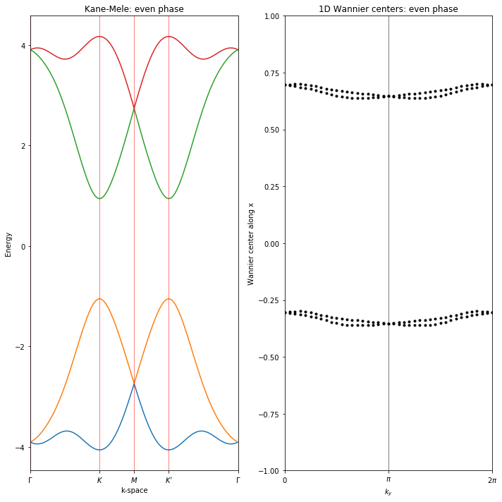
Kane-Mele model using spinor features
#!/usr/bin/env python
# Two dimensional tight-binding 2D Kane-Mele model
# C.L. Kane and E.J. Mele, PRL 95, 146802 (2005) Eq. (1)
from __future__ import print_function
from pythtb import * # import TB model class
import numpy as np
import matplotlib.pyplot as plt
def get_kane_mele(topological):
"Return a Kane-Mele model in the normal or topological phase."
# define lattice vectors
lat = [[1.0,0.0],[0.5,np.sqrt(3.0)/2.0]] # 二维元胞基矢
# define coordinates of orbitals
orb = [[1./3.,1./3.],[2./3.,2./3.]] # 元胞中轨道的位置
# make two dimensional tight-binding Kane-Mele model
ret_model = tbmodel(2,2,lat,orb,nspin = 2) # 实空间与动量空间都是2维,且此时考虑了自旋
# set model parameters depending on whether you are in the topological
# phase or not
# 不同的参数值决定体系是拓扑或者非拓扑
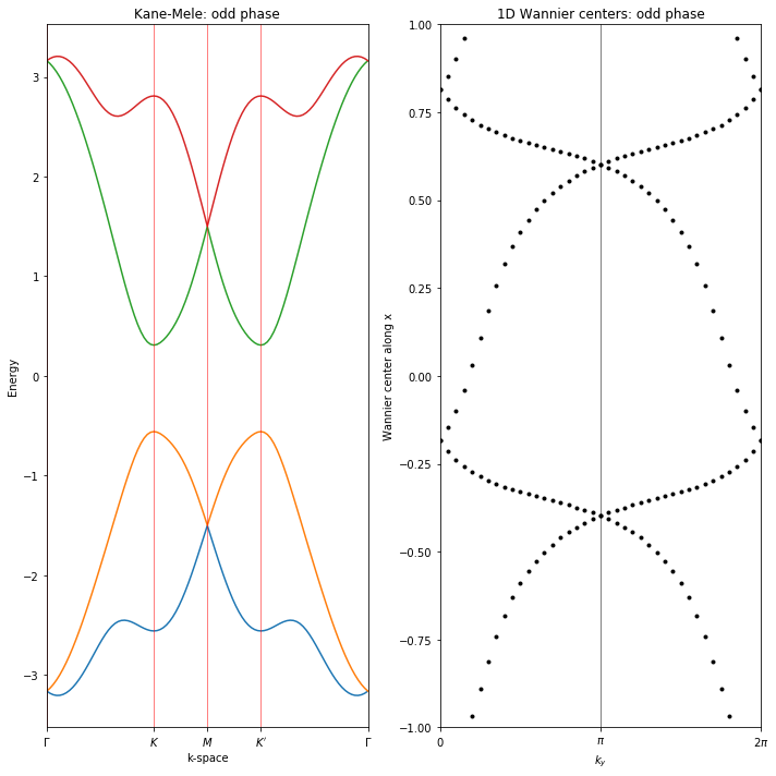
if topological=="even":
esite = 2.5
elif topological=="odd":
esite = 1.0
# set other parameters of the model
thop = 1.0
spin_orb = 0.6*thop*0.5
rashba = 0.25*thop
# set on-site energies
ret_model.set_sites([esite,(-1.0)*esite])
# set hoppings (one for each connected pair of orbitals)
# (amplitude, i, j, [lattice vector to cell containing j])
# useful definitions
# 定义泡里矩阵
sigma_x = np.array([0.,1.,0.,0])
sigma_y = np.array([0.,0.,1.,0])
sigma_z = np.array([0.,0.,0.,1])
# spin-independent first-neighbor hoppings
ret_model.set_hop(thop, 0, 1, [ 0, 0])
ret_model.set_hop(thop, 0, 1, [ 0,-1])
ret_model.set_hop(thop, 0, 1, [-1, 0])
# second-neighbour spin-orbit hoppings (s_z)
ret_model.set_hop(-1.j*spin_orb*sigma_z, 0, 0, [ 0, 1])
ret_model.set_hop( 1.j*spin_orb*sigma_z, 0, 0, [ 1, 0])
ret_model.set_hop(-1.j*spin_orb*sigma_z, 0, 0, [ 1,-1])
ret_model.set_hop( 1.j*spin_orb*sigma_z, 1, 1, [ 0, 1])
ret_model.set_hop(-1.j*spin_orb*sigma_z, 1, 1, [ 1, 0])
ret_model.set_hop( 1.j*spin_orb*sigma_z, 1, 1, [ 1,-1])
# Rashba first-neighbor hoppings: (s_x)(dy)-(s_y)(d_x)
r3h = np.sqrt(3.0)/2.0
# bond unit vectors are (r3h,half) then (0,-1) then (-r3h,half)
ret_model.set_hop(1.j*rashba*( 0.5*sigma_x - r3h*sigma_y), 0, 1, [ 0, 0], mode = "add") # 在最近邻格点上增加自旋轨道耦合项
ret_model.set_hop(1.j*rashba*(-1.0*sigma_x ), 0, 1, [ 0,-1], mode = "add")
ret_model.set_hop(1.j*rashba*( 0.5*sigma_x + r3h*sigma_y), 0, 1, [-1, 0], mode = "add")
return ret_model
# now solve the model and find Wannier centers for both topological
# and normal phase of the model
for top_index in ["even","odd"]:
# get the tight-binding model
my_model = get_kane_mele(top_index)
# list of nodes (high-symmetry points) that will be connected
path = [[0.,0.],[2./3.,1./3.],[.5,.5],[1./3.,2./3.], [0.,0.]] # 构造需要进行计算的路径
# labels of the nodes
label=(r'$\Gamma $',r'$K$', r'$M$', r'$K^\prime$', r'$\Gamma $')
(k_vec,k_dist,k_node) = my_model.k_path(path,101,report=False)
# initialize figure with subplots
fig, (ax1, ax2) = plt.subplots(1,2,figsize=(10,10))
# solve for eigenenergies of hamiltonian on
# the set of k-points from above
evals = my_model.solve_all(k_vec) # 在上面求得的k点上进行模型计算
# plot bands
ax1.plot(k_dist,evals[0])
ax1.plot(k_dist,evals[1])
ax1.plot(k_dist,evals[2])
ax1.plot(k_dist,evals[3])
ax1.set_title("Kane-Mele: " + top_index + " phase")
ax1.set_xticks(k_node)
ax1.set_xticklabels(label)
ax1.set_xlim(k_node[0],k_node[-1])
for n in range(len(k_node)):
ax1.axvline(x = k_node[n],linewidth = 0.5, color = 'r') # 做标记的竖线
ax1.set_xlabel("k-space")
ax1.set_ylabel("Energy")
#calculate my-array
my_array = wf_array(my_model,[41,41]) # 计算波函数
# solve model on a regular grid, and put origin of
# Brillouin zone at [-1/2,-1/2] point
my_array.solve_on_grid([-0.5,-0.5]) # 在给定的k点上求解TB模型
# calculate Berry phases around the BZ in the k_x direction
# (which can be interpreted as the 1D hybrid Wannier centers
# in the x direction) and plot results as a function of k_y
#
# Following the ideas in
# A.A. Soluyanov and D. Vanderbilt, PRB 83, 235401 (2011)
# R. Yu, X.L. Qi, A. Bernevig, Z. Fang and X. Dai, PRB 84, 075119 (2011)
# the connectivity of these curves determines the Z2 index
#
wan_cent = my_array.berry_phase([0,1],dir=1,contin=False,berry_evals=True) # 计算前两个能带的Berry位相
wan_cent /= (2.0*np.pi)
nky = wan_cent.shape[0]
ky = np.linspace(0.,1.,nky)
# draw shifted Wannier center positions
for shift in range(-2,3):
ax2.plot(ky,wan_cent[:,0] + float(shift),"k.")
ax2.plot(ky,wan_cent[:,1] + float(shift),"k.")
ax2.set_ylim(-1.0,1.0)
ax2.set_ylabel('Wannier center along x')
ax2.set_xlabel(r'$k_y$')
ax2.set_xticks([0.0,0.5,1.0])
ax2.set_xlim(0.0,1.0)
ax2.set_xticklabels([r"$0$",r"$\pi$", r"$2\pi$"])
ax2.axvline(x=.5,linewidth=0.5, color='k')
ax2.set_title("1D Wannier centers: "+top_index+" phase")
fig.tight_layout()
fig.savefig("kane_mele_"+top_index+".pdf")
print('Done.\n')
Done.
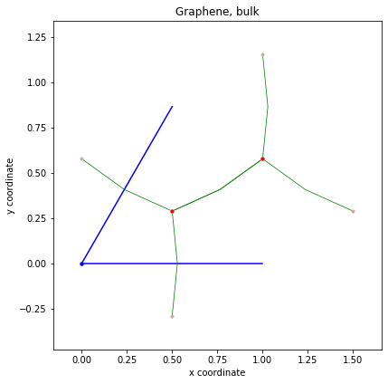
Visualization example
#!/usr/bin/env python
# Visualization example
from __future__ import print_function
from pythtb import * # import TB model class
import numpy as np
# define lattice vectors
lat = [[1.0,0.0],[0.5,np.sqrt(3.0)/2.0]]
# define coordinates of orbitals
orb = [[1./3.,1./3.],[2./3.,2./3.]]
# make two dimensional tight-binding graphene model
my_model = tb_model(2,2,lat,orb)
# set model parameters
delta = 0.0
t = -1.0
# set on-site energies
my_model.set_onsite([-delta,delta])
# set hoppings (one for each connected pair of orbitals)
# (amplitude, i, j, [lattice vector to cell containing j])
my_model.set_hop(t, 0, 1, [ 0, 0])
my_model.set_hop(t, 1, 0, [ 1, 0])
my_model.set_hop(t, 1, 0, [ 0, 1])
# visualize infinite model
(fig,ax) = my_model.visualize(0,1) #显示所有的轨道
ax.set_title("Graphene, bulk")
ax.set_xlabel("x coordinate")
ax.set_ylabel("y coordinate")
fig.tight_layout()
fig.savefig("visualize_bulk.pdf")
# cutout finite model along direction 0
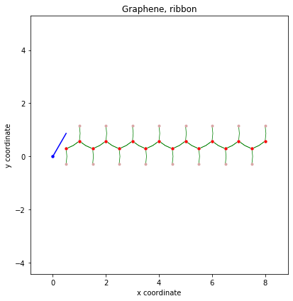
cut_one = my_model.cut_piece(8,0,glue_edgs = False) # x方向重复8个元胞
#
(fig,ax) = cut_one.visualize(0,1)
ax.set_title("Graphene, ribbon")
ax.set_xlabel("x coordinate")
ax.set_ylabel("y coordinate")
fig.tight_layout()
fig.savefig("visualize_ribbon.pdf")
# cutout finite model along direction 1 as well
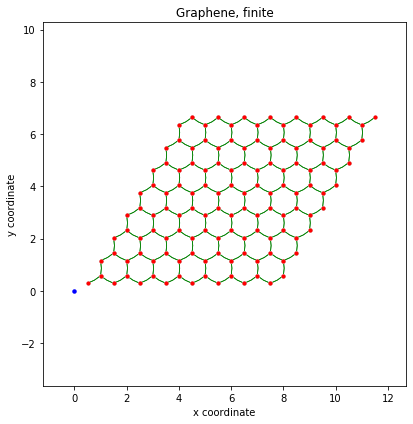
cut_two = cut_one.cut_piece(8,1,glue_edgs = False) # x,y方向同时取8个重复结构
#
(fig,ax) = cut_two.visualize(0,1)
ax.set_title("Graphene, finite")
ax.set_xlabel("x coordinate")
ax.set_ylabel("y coordinate")
fig.tight_layout()
fig.savefig("visualize_finite.pdf")
print('Done.\n')
Done.
公众号
相关内容均会在公众号进行同步,若对该Blog感兴趣,欢迎关注微信公众号。

|
yxli406@gmail.com |