Fortran + Gnu 批量计算
做模型研究的时候,通常会调节一个模型的很多参数来研究这些参数变化时某些量是如何演化的,这就涉及到批量计算绘图的问题,我是习惯用Fortran了,因为计算速度比较快,而且自己也比较熟悉了,结合gnuplot可以快速的将不同数据对应的结果进行作图.这里的有些内容可以参考做数值计算好用的软件及杂项整理这篇中的内容,废话不多说,直接上代码进行解释.
Fortran + Gnuplot 批量数据输出绘图
1 | ! Anticommute mass term along y open gap |
上面代码主要的内容是1
2
3
4
5
6
7
8
9
10
11
12
13
14
15
16
17
18
19
20
21
22
23
24
25
26
27
28
29
30
31
32
33 subroutine cylinder(m3)
! Calculate edge spectrum function
use pub
integer m1,m2,m3
real kx,ky
character*20::str1,str2,str3,str4,str5,str6
str1 = "oy45-sc-ym"
str2 = "ox45-sc-ym"
write(str3,"(I2.2)")m3
str4 = ".dat"
str5 = trim(str1)//trim(str3)//trim(str4)
str6 = trim(str2)//trim(str3)//trim(str4)
open(30,file=str5)
!-------------------------------------------------
! y-direction is open
do m1 = -kn,kn
kx = pi*m1/kn
call openy(kx)
write(30,999)kx/pi,(w(i),i = 1,N)
end do
close(30)
!--------------------------------------------------
! x-direction is open
open(31,file=str6)
do m1 = -kn,kn
ky = pi*m1/kn
call openx(ky)
write(31,999)ky/pi,(w(i),i=1,N)
end do
close(31)
999 format(802f11.5)
return
end subroutine cylinder
通过下面的代码可以组合出随着m3变化的字符串,将其作为文件名,这样就会对不同的输出,产生相对应的数据文件1
2
3
4
5
6str1 = "oy45-sc-ym"
str2 = "ox45-sc-ym"
write(str3,"(I2.2)")m3
str4 = ".dat"
str5 = trim(str1)//trim(str3)//trim(str4)
str6 = trim(str2)//trim(str3)//trim(str4)
而在绘图部分1
2
3
4
5
6
7
8
9
10
11
12
13
14
15
16
17
18
19
20
21
22
23
24
25
26
27
28
29
30
31subroutine plot(m3)
use pub
character*20::str1,str2,str3,str4,str5,str6
integer m3
str1 = "diag-ym"
write(str2,"(I2.2)")m3
str3 = ".gnu"
str4 = trim(str1)//trim(str2)//trim(str3)
open(20,file=str4)
write(20,*)'set terminal png truecolor enhanced font ",50" size 3000, 1500'
write(20,*)"set output 'diag"//trim(str2)//"-cy-ym.png'"
write(20,*)"set size 1, 1"
write(20,*)"set multiplot layout 1, 2"
write(20,*)"unset key"
write(20,*)"set ytics 1.5 "
write(20,*)"set xtics 0.5"
write(20,*)"set xtics offset 0, 0.0"
write(20,*)'set xtics format "%4.1f" nomirror out '
write(20,*)'set ytics format "%4.1f"'
write(20,*)'set ylabel "E"'
write(20,*)"set ylabel offset 0.5, 0.0 "
write(20,*)"#set xlabel offset 0, -1.0 "
write(20,*)"set xrange [-1:1]"
write(20,*)"set yrange [-3:3]"
write(20,*)"set xlabel 'k_y' "
write(20,*)"plot for [i=2:400] 'ox45-sc-ym"//trim(str2)//".dat' u 1:i w l lw 5 lc 'blue'"
write(20,*)"set xlabel 'k_x' "
write(20,*)"plot for [i=2:400] 'oy45-sc-ym"//trim(str2)//".dat' u 1:i w l lw 5 lc 'blue'"
write(20,*)"unset multiplot"
close(20)
end subroutine plot
同样利用相同的方法来产生相对应数据的gnuplot作图文件.
这里再提供一个编译执行fortran文件的shell脚本1
2
3
4
5
6
7
8
9
10!/bin/sh
============ get the file name ===========
rm *.gnu *.png no* *.dat *.out 1>/dev/null 2>/dev/null &
Folder_A=$(pwd)
for file_a in ${Folder_A}/*.f90
do
temp_file=`basename $file_a .f90`
ifort -mkl -O3 -CB $file_a -o $temp_file.out
nohup ./$temp_file.out 1>/dev/null 2>/dev/null &
done
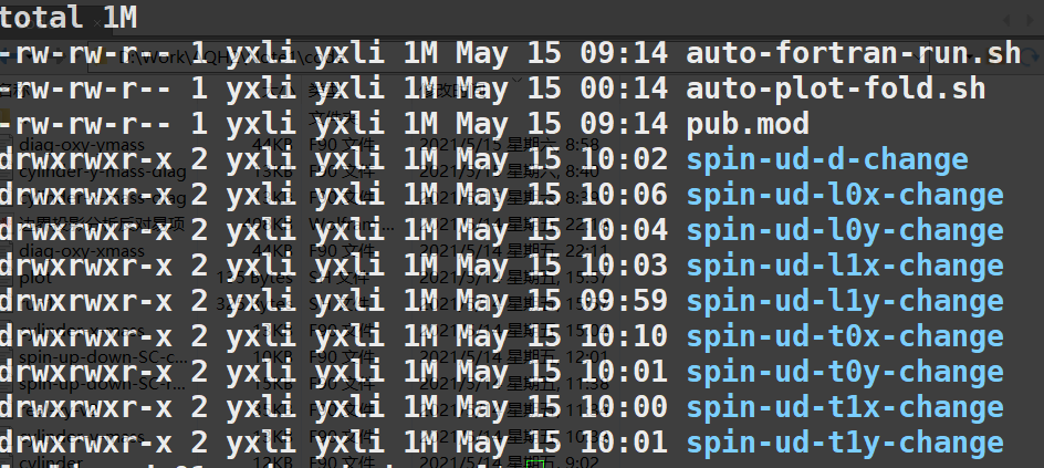
将上面的脚本命名为run1.sh然后执行1
sh run1.sh
结果如下图所示
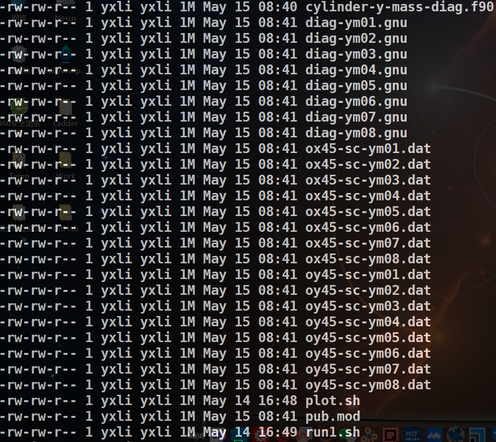
可以看到这里得到了数据结果filename.dat与其相应的一系列绘图脚本filename.gnu,下面批量执行所有的filename.gnu绘图脚本1
2
3
4
5
6
7!/bin/sh
============ get the file name ===========
Folder_A=$(pwd)
for file_a in ${Folder_A}/*.gnu
do
gnuplot $file_a
done
同样的,这个脚本的作用是寻找该文件夹下面所有后缀为.gnu的文件,执行绘图程序gnuplot filename.gnu,结果如下
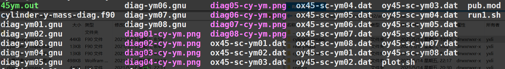
可以看到批量执行之后会有一系列的结果图.
文件夹递归操作
除了对单个文件夹中的多个文件进行编译执行操作,有时候在计算时,可能会有很多个文件夹,而每个文件夹中又有多个文件需要进行编译执行,这时候上面的脚本就不能发挥作用了,需要对文件夹进行递归操作,也就是说要找到当前文件夹下面包含的每个文件夹,进行该文件夹然后再执行上面的脚本,比如当前文件夹下面还有一些文件夹
1 | !/bin/bash |
代码的主要部分是1
2
3
4
5dir1 # 切换到具体的文件夹
sh run1.sh & # 执行当前文件夹下面的run1.sh脚本
./$file_name.out 1>mes 2>bad & # 执行该文件夹下面编译好的文件
./$out_file_name.out 1>mes 2>bad &
rm $out_file_name.out
我在这里使用了sh run1.sh这个命令,这样的好处是会对cd切换到的每个文件夹中均编译执行所有.f90的文件(这是脚本run1.sh的功能),同样也可以使用1
2./$file_name.out 1>mes 2>bad & # 执行该文件夹下面编译好的文件
./$out_file_name.out 1>mes 2>bad &
这个命令,我这里是将它进行了注释,它也是会编译并执行所有后缀为.f90的文件,而关于后缀名的选择,是在1
if [ "${dir_or_file##*.}"x = "f90"x ]||[ "${dir_or_file##*.}"x = "f"x ];then # 筛选处特定后缀的文件
这里进行筛选的,所以如果是想要编译执行其他类型程序的文件,可以对这个后缀名进行修改并调整对应的编译器即可.
在将fortran程序递归的编译执行完成之后,每个文件夹中会产生了许多的.gnu文件可以用来绘图,与上面相同的思路,此时递归遍历每个文件夹并执行plot.sh这个绘图脚本1
2
3
4
5
6
7
8
9
10
11
12
13
14
15
16
17
18
19
20
21
22
23
24
25
26
27
28
29!/bin/bash
function getdir(){
for element in `ls $1`
do
dir_or_file=$1"/"$element
if [ -d $dir_or_file ]
then
getdir $dir_or_file
else # 下面的全是文件
if [ "${dir_or_file##*.}"x = "gnu"x ];then # 筛选处特定后缀的文件
dir_name=`dirname $dir_or_file` # 读取目录
file_name=`basename $dir_or_file .gnu` # 读取以.gnu结尾的文件名
out_file_name="$dir_name/$file_name" # 定义编号成功的文件名称
ifort -mkl $dir_or_file -o $out_file_name.out # 编译后文件名以out结尾
dir1=`dirname $out_file_name`
echo $dir1
cd $dir1 # 切换到具体的文件夹
gnuplot $dir_or_file &
fi
#temp_file=`basename $dir_or_file .f90` #将文件名后缀删除
#ifort -mkl $dir_or_file -o $temp_file.out # 编译后文件名以out结尾
#echo $dir_or_file # 这里的变量时完整的路径名
fi
done
}
fold="/home/yxli/te"
fold=`pwd`
getdir $fold
最终就可以将所有文件夹下面的程序执行完毕,并进行绘图了.
小改动
这里稍微修改了一下程序编译后的名称,干脆用数字表示了,防止因为原来的文件名太长,导致可执行文件名也很长,不方便查看.1
2
3
4
5
6
7
8
9
10
11
12
13
14
15
16
17
18
19
20
21
22
23
24
25
26
27
28
29
30
31
32
33
34
35
36
37
38!/bin/bash
递归搜寻文件夹下面所有的.f90或者.f后缀结尾的文件,并利用ifort编译该文件,然后执行
cnt=0 # 定义一个变量,来统计文件夹下面对应程序的个数
function getdir(){
for element in `ls $1`
do
out="out"
dir_or_file=$1"/"$element
if [ -d $dir_or_file ]
then
getdir $dir_or_file
else # 下面的全是文件
rm *dat *gnu *png 1>/dev/null 2>/dev/null
if [ "${dir_or_file##*.}"x = "f90"x ]||[ "${dir_or_file##*.}"x = "f"x ];then # 筛选处特定后缀的文件
cnt=$[$cnt+1]
dir_name=`dirname $dir_or_file` # 读取目录
file_name=`basename $dir_or_file .f90` # 读取以f90结尾的文件名
out_file_name="$dir_name/$file_name" # 定义编号成功的文件名称
out_file_name="$dir_name/$cnt" # 定义编号成功的文件名称
ifort -mkl $dir_or_file -o $out_file_name.$out # 开始编译fortran文件,编译后文件名以out结尾,以数字命名
dir1=`dirname $out_file_name`
echo $out_file_name.$out
echo $dir1
cd $dir1 # 切换到具体的文件夹,是为了在具体的文件夹中,运行编译好的可执行文件
echo $cnt.$out
./$cnt.$out 1>/dev/null 2>/dev/null & # 执行该文件夹下面编译好的文件
rm $out_file_name.$out
fi
#temp_file=`basename $dir_or_file .f90` #将文件名后缀删除
#ifort -mkl $dir_or_file -o $temp_file.out # 编译后文件名以out结尾
#echo $dir_or_file # 这里的变量时完整的路径名
fi
done
}
root_dir=`pwd`
getdir $root_dir
鉴于该网站分享的大都是学习笔记,作者水平有限,若发现有问题可以发邮件给我
- yxliphy@gmail.com
也非常欢迎喜欢分享的小伙伴投稿


欢迎关注公众号,有趣的内容也会在上面同步。 有密码的文章属于正在建设中或者没有通过验证的内容,若有需要可通过邮件联系。

![超导自由能泛函(Ginzburg–Landau)推导[非均匀配对]](/assets/images/SC/SC-Free.png)