快速格林函数方法计算Chern绝缘体边界态
这篇博客整理一下如何利用格林函数方法来计算Chern绝缘体不同边界上的边界态.
{:.info}
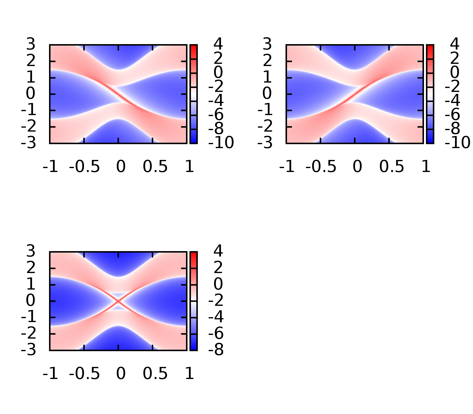
在Chern Insulator边界态及Chern数计算这篇博客中提供了计算Chern绝缘体边界态的程序,但是因为那个方法中是在一个cylinder上进行计算的,所以会存在两个边界,从而也就会在能谱中看到有两个边界态,这在有时候的研究中是不太方便的,这里就像通过格林函数的方法,计算一个半无限大的系统,因为只存在一个边界,所以对于Chern绝缘体来说此时就可以得到只有一个边界态的能谱图,而且还可以分别计算左右两端的边界态,可以发现其对应的费米速度是相反的.
计算公式
这里使用的就是Highly convergent schemes for the calculation of bulk and surface Green functions这篇文章中的计算方法,不过需要对写程序中一些具体内容进行一下说明.
当将一个动量空间中的哈密顿量沿某一个方向取开边界,另一个方向取周期边界的时候,对应的哈密顿量矩阵为
因为哈密顿量是厄米的,所以就会有$H_{01}=H_{i,i+1}=H^\dagger_{i+1,i},H_{00}=H_{ii}=H_{i+1.i+1}$.
想要得到格林函数
可以通过下面的迭代方程进行
初始值的选择为$\epsilon_0=H_{00},\alpha_0=H_{01},\beta_0=H^\dagger_{01}$.通过一定的迭代循环之后就可以得到对应的$\epsilon^s,\epsilon$.利用这两个得到的值就可以计算哈密顿量对应的边界态,
上面计算的是一端的边界态,如果想计算另外一端的边界态,需要对迭代进行修改
即可,计算结果如下
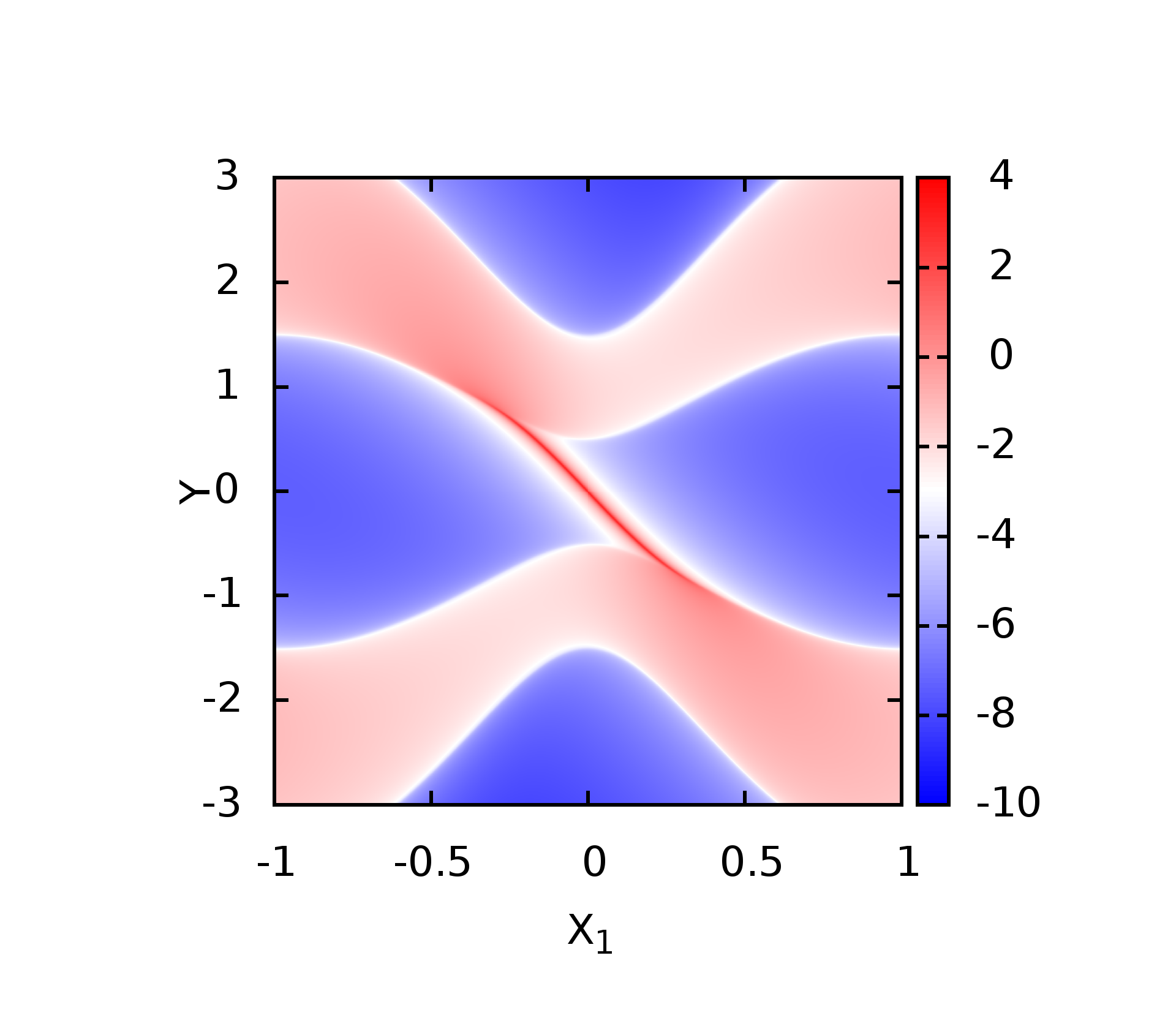
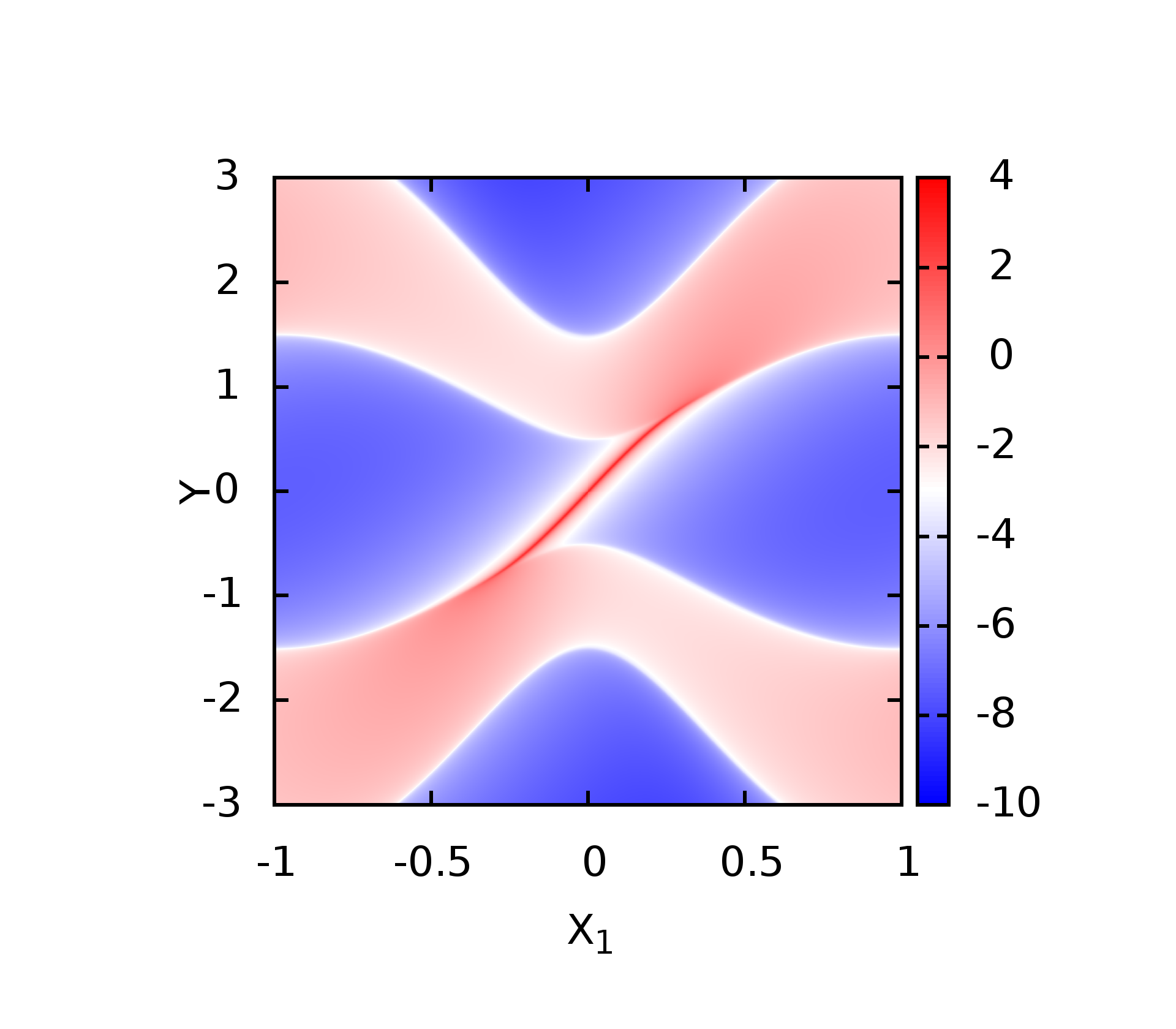

这里的第三张是将两个边界态同时计算的结果.
代码
Julia
1 | using LinearAlgebra,DelimitedFiles,PyPlot |
- 首先通过julia计算得到对应的数据
1 | program main |
- 接下来通过fortran来将数据进行格式化之后,准备作图
1 | set encoding iso_8859_1 |
- 最后利用gnuplot进行图形绘制即可
Fortran
同样可以利用Fortran来进行计算1
2
3
4
5
6
7
8
9
10
11
12
13
14
15
16
17
18
19
20
21
22
23
24
25
26
27
28
29
30
31
32
33
34
35
36
37
38
39
40
41
42
43
44
45
46
47
48
49
50
51
52
53
54
55
56
57
58
59
60
61
62
63
64
65
66
67
68
69
70
71
72
73
74
75
76
77
78
79
80
81
82
83
84
85
86
87
88
89
90
91
92
93
94
95
96
97
98
99
100
101
102
103
104
105
106
107
108
109
110
111
112
113
114
115
116
117
118
119
120
121
122
123
124
125
126
127
128
129
130
131
132
133
134
135
136
137
138
139
140
141
142
143
144
145
146
147
148
149
150
151
152
153
154
155
156
157
158
159
160
161
162
163
164
165
166
167
168
169
170
171
172
173
174
175
176
177
178
179 module pub
implicit none
integer N,iternum,hn
real err,eta,dk,domg
parameter( hn = 2, N = hn,iternum = 200,err = 1e-16,eta = 0.01,dk = 0.01,domg = dk)
real,parameter::pi = 3.1415926535
complex,parameter::im = (0.,1.0)
complex ones(N,N),GLL(N,N),GRR(N,N),GB(N,N)
complex H00(N,N) ! diagonal elementery
complex H01(N,N) ! off-diag elementery
complex g1(hn,hn),g2(hn,hn),g3(hn,hn)
!---------------------------------------------
real m0,mu
real tx,ty
real ax,ay
end module pub
!==================================================================
program main
use pub
!======parameter value setting =====
m0 = 1.5
tx = 1.0
ty = 1.0
ax = 1.0
ay = 1.0
call surfstat()
stop
end program main
!============================================================================================
subroutine surfstat()
! surfstat calculates surface state using green's function method---J.Phys.F.Met.Phys.15(1985)851-858
! 利用已经求得的格林函数来计算对应的态密度
use pub
implicit none
real kx,omg,re1,re2,re3
real t_start,t_end
integer i1
open(20,file="dos.dat")
call cpu_time(t_start)
!------------------------------------------
do kx = -pi,pi,dk
call matset(kx)
do omg = -3,3,domg
call itera(omg,kx)
re1 = log(abs(sum(aimag(GLL))))
re2 = log(abs(sum(aimag(GRR))))
re3 = log(abs(sum(aimag(GB))))
write(20,999)kx/pi,omg,re1,re2,re3
end do
write(20,*)" "
end do
!------------------------------------------
call cpu_time(t_end)
close(20)
write(*,*)"Timing const is: ",t_end - t_start
999 format(30f16.12)
return
end subroutine surfstat
!=================================================================
subroutine itera(omega,ky)
use pub
real omega,real_temp,ky
integer iter
complex omegac
complex g0dem(N,N), g0(N,N) ! Green's Function
complex epsiloni(N,N),epsilons(N,N),epsilons_t(N,N),alphai(N,N),betai(N,N) ! 迭代过程变量
complex GLLdem(N,N),GRRdem(N,N),GBdem(N,N),mat1(N,N),mat2(N,N)
!----------------------------
call matset(ky)
epsiloni = H00
epsilons = H00
epsilons_t = H00
alphai = H01
betai = conjg(transpose(H01))
omegac = omega + eta*im
!----------------------------------
do iter = 1, iternum
g0dem = omegac*ones - epsiloni ! Green's Function
call inv(g0dem, g0)
mat1 = matmul(alphai, g0)
mat2 = matmul(betai, g0)
g0 = matmul(mat1,betai)
epsiloni = epsiloni + g0
epsilons = epsilons + g0
g0 = matmul(mat2,alphai)
epsiloni = epsiloni + g0
epsilons_t = epsilons_t + g0
g0 = matmul(mat1, alphai)
alphai = g0
g0 = matmul(mat2, betai)
betai = g0
real_temp = sum(abs(alphai))
if (real_temp .le. err)then
exit
end if
end do ! end of iteration
! calculate surface green's function
GLLdem = omegac*ones- epsilons
call inv(GLLdem, GLL)
! GLL = epsilons
GRRdem = omegac*ones- epsilons_t
call inv(GRRdem, GRR)
! GRR = epsilons_t
GBdem = omegac*ones- epsiloni
call inv(GBdem, GB)
! GB = epsiloni
end subroutine itera
!================================================================
subroutine matset(ky)
! 构建哈密顿量
use pub
real ky
integer m,l
call Pauli()
do m = 1,hn
do l = 1,hn
H00(m,l) = (m0-ty*cos(ky))*g1(m,l) + ay*sin(ky)*g3(m,l)
H01(m,l) = (-tx*g1(m,l) - im*ax*g2(m,l))/2
end do
end do
!----------------------
! 初始化单位矩阵
do ix = 1,N
ones(ix,ix) = 1.0
end do
return
end subroutine matset
!=======================矩阵求逆====================================
subroutine inv(matin,matout)
use pub
complex,intent(in) :: matin(N,N) ! N is dimension of matrix which can be readed from pub model (use pub)
complex:: matout(size(matin,1),size(matin,2))
real:: work2(size(matin,1)) ! work2 array for LAPACK
integer::ipiv(size(matin,1)) ! pivot indices
integer info ! inv solution information
! Store matin in matout to prevent it from being overwritten by LAPACK
matout = matin
! SGETRF computes an LU factorization of a general M-by-N matrix A
! using partial pivoting with row interchanges.
call CGETRF(N,N,matout,N,ipiv,info)
if (info.ne.0) stop 'Matrix is numerically singular!'
! SGETRI computes the inverse of a matrix using the LU factorization
! computed by SGETRF.
call CGETRI(N,matout,N,ipiv,work2,N,info)
if (info.ne.0) stop 'Matrix inversion failed!'
return
end subroutine inv
!====================================================
subroutine Pauli()
use pub
!----------
g1(1,1) = 1
g1(2,2) = -1
!----------
g2(1,2) = 1
g2(2,1) = 1
!----------
g3(1,2) = -im
g3(2,1) = im
return
end subroutine Pauli
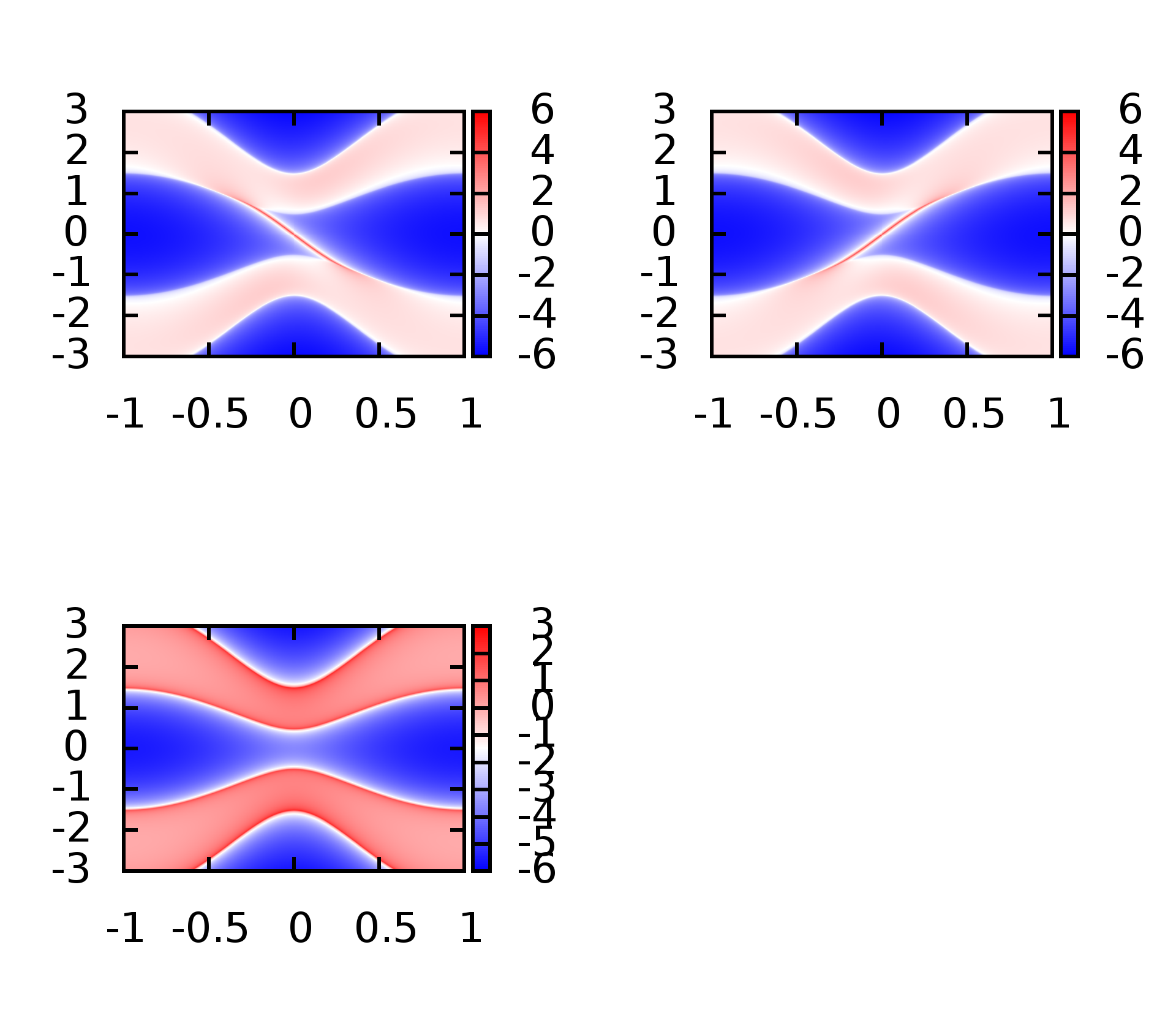
此时可以同时计算出左边界,有边界以及体态的能带.
补充
上面是将三张分开绘制的,利用的分别是数据的第三,第四,第五列,这里将三个结果绘制到统一张图上1
2
3
4
5
6
7
8
9
10
11
12
13
14
15
16
17
18
19
20
21
22
23
24
25
26
27
28
29
30
31
32
33set encoding iso_8859_1
set terminal postscript enhanced color
set output 'arc_r.eps'
set terminal pngcairo truecolor enhanced font ",50" size 1920, 1680
set terminal png truecolor enhanced font ",50" size 1920, 1680
set output 'Chern.png'
set size 2, 1
set palette defined ( -10 "#194eff", 0 "white", 10 "red" )
set palette defined ( -10 "blue", 0 "white", 10 "red" )
set palette rgbformulae 33,13,10
set multiplot layout 2,2
unset ztics
unset key
set pm3d
set border lw 6
set size ratio 1
set view map
set xtics
set ytics
set xlabel "K_1 (1/{\305})"
set xlabel "X_1"
set ylabel "K_2 (1/{\305})"
set ylabel "Y"
set ylabel offset 1, 0
set colorbox
set xrange [-1:1]
set yrange [-3:3]
set pm3d interpolate 4,4
splot 'wavenorm.dat' u 1:2:3 w pm3d
splot 'wavenorm.dat' u 1:2:3 w pm3d
splot 'test-format.dat' u 1:2:3 w pm3d
splot 'test-format.dat' u 1:2:4 w pm3d
splot 'test-format.dat' u 1:2:5 w pm3d
Python Version
最近搞科研,发现许多函数还是使用python比较好,借用其比较好的生态,想要实现某些功能不需要自己去写相对应的函数1
2
3
4
5
6
7
8
9
10
11
12
13
14
15
16
17
18
19
20
21
22
23
24
25
26
27
28
29
30
31
32
33
34
35
36
37
38
39
40
41
42
43
44
45
46
47
48
49
50
51
52
53
54
55
56
57
58
59
60
61
62
63
64
65
66
67
68
69
70
71
72
73
74
75
76
77
78
79
80
81
82
83
84
85
86
87
88
89
90
91
92
93
94
95
96
97
98
99
100
101
102
103
104
105
106
107
108
109
110
111
112
113
114
115
116
117
118
119
120
121
122
123
124
125
126
127
128
129
130
131
132
133
134
135
136
137
138
139
140
141import numpy as np
import matplotlib.pyplot as plt
import os
import time
import seaborn as sns
def Pauli():
s0 = np.array([[1,0],[0,1]])
sx = np.array([[0,1],[1,0]])
sy = np.array([[0,-1j],[1j,0]])
sz = np.array([[1,0],[0,-1]])
return s0,sx,sy,sz
#------------------------------------------------
def hamset(ki):
m0 = 1.5
tx = 1.0
ty = 1.0
ax = 1.0
ay = 1.0
s0,sx,sy,sz = Pauli()
H00 = np.zeros((2,2),np.complex128)
H01 = np.zeros((2,2),np.complex128)
for i0 in range(2):
for i1 in range(2):
H00[i0,i1] = (m0 - tx*np.cos(ki))*sz[i0,i1] + ax*np.sin(ki)*sx[i0,i1]
H01[i0,i1] = -ty/2.0*sz[i0,i1] + ay/(2.0*1j)*sy[i0,i1]
return H00,H01
# -----------------------------------------------------------------------
def Iteration(omega,ki):
err = 1e-16
eta = 0.01
iternum = 200
H00 = np.zeros((2,2),np.complex128)
H01 = np.zeros((2,2),np.complex128)
H00,H01 = hamset(ki)
epsiloni = H00
epsilons = H00
epsilons_t = H00
alphai = H01
betai = H01.T.conjugate() # 转置共轭
omegac = omega + eta*1j
s0,sx,sy,sz = Pauli()
for i0 in range(iternum):
g0dem = omegac*s0 - epsiloni
g0 = np.linalg.inv(g0dem)
mat1 = np.dot(alphai,g0)
mat2 = np.dot(betai,g0)
g0 = np.dot(mat1,betai)
epsiloni = epsiloni + g0
epsilons = epsilons + g0
g0 = np.dot(mat2,alphai)
epsiloni = epsiloni + g0
epsilons_t = epsilons_t + g0
g0 = np.dot(mat1, alphai)
alphai = g0
g0 = np.dot(mat2,betai)
betai = g0
real_temp = np.sum(np.concatenate(np.abs(alphai)))
if (real_temp < err):
break
GLLdem = omegac*s0 - epsilons
GLL = np.linalg.inv(GLLdem)
# GLL = epsilons
GLL = np.sum(np.concatenate(np.abs(GLL)))
GRRdem = omegac*s0 - epsilons_t
GRR = np.linalg.inv(GRRdem)
GRR = np.sum(np.concatenate(np.abs(GRR)))
# GRR = epsilons_t
GBdem = omegac*s0 - epsiloni
GB = np.linalg.inv(GBdem)
GB = np.sum(np.concatenate(np.abs(GB)))
# GB = epsiloni
return GLL,GRR,GB
#------------------------------------------------------------
def surface():
nx = 100
max_omg = 1.5
re = np.zeros((len(range(-nx,nx))**2,5))
con = 0
ix = -1
iy = -1
GLL = np.zeros((len(range(-nx,nx)),len(range(-nx,nx))))
GRR = np.zeros((len(range(-nx,nx)),len(range(-nx,nx))))
GB = np.zeros((len(range(-nx,nx)),len(range(-nx,nx))))
for i0 in range(-nx,nx):
kx = np.pi*i0/nx
for i1 in range(-nx,nx):
omg = max_omg*i1/nx
re1,re2,re3 = Iteration(omg,kx)
re[con,0] = kx
re[con,1] = omg
re[con,2] = re1
re[con,3] = re2
re[con,4] = re3
GLL[iy,ix] = np.log(re1)
GRR[iy,ix] = np.log(re2)
GB[iy,ix] = np.log(re3)
con += 1
iy += 1
ix += 1
iy = 0
# np.savetxt("GLL.dat", [kilist,re1list], fmt="%15.10f")
# np.savetxt("GRR.dat", [kilist,re1list], fmt="%15.10f")
# np.savetxt("GB.dat", [kilist,re1list], fmt="%15.10f")
np.savetxt("density.dat",re , fmt="%15.10f")
return GLL,GRR,GB
#-----------------------------------------------------------------------
def main():
os.chdir(os.getcwd())
tstart = time.time()
GLL,GRR,GB = surface()
tend = time.time()
#print(tend - tstart)
# 绘图
sns.set()
ax = sns.heatmap(GB)
plt.show()
#-----------------------------------------------------------------------
if __name__ == '__main__':
main()
这里最终计算的结果肯定是相同的,只不过绘图的时候给出的横纵坐标我没有去设置,这个具体使用的时候,到后面再去慢慢调整。
参考
公众号
相关内容均会在公众号进行同步,若对该Blog感兴趣,欢迎关注微信公众号。
{:.info}

|
yxliphy@gmail.com |
 wechat
 alipay