根据对称性计算体系电四极矩
模型
这里研究我最熟悉的模型,将BHZ模型和$d$波超导体结合起来,这早期实现高阶拓扑超导体的方案之一,其模型为
这个是一个体态电四极矩贡献的高阶拓扑相(这里我就不解释为什么了,感兴趣可以和我讨论)。它具有$x$和$y$方向的Mirror对称性
哈密顿量在Mirror对称操作下满足
除此之外系统还存在inverison对称性
当体系存在Mirror对称性和空间反演对称性之后,其Wannier sector的极化满足(可以参考Electric multipole moments, topological multipole moment pumping, and chiral hinge states in crystalline insulators这篇文章)
所以,如果存在$\mathcal{M}_x,\mathcal{M}_y,\mathcal{P}$的时候,$p_y^{\theta_x^{\pm}}$一定会是量子化的
此时可以通过对称操作在高对称点的本征值来计算Wannier sector的极化(参考Electric multipole moments, topological multipole moment pumping, and chiral hinge states in crystalline insulators),此时Wannier band basis(参考Nested Wilson loop)满足
这里$\alpha^{\pm}_{M_y}(k_x,k_y)$是$U(1)$的位相。
在reflection不变动量点$k_{y}=0 \text{ 和 }\pi$上,$\alpha^{\pm}_{M_y}(k_x, k_{y})$ 是 $\rvert w^\pm_{x,\bf k}\rangle$ 在 $(k_x,k_{*y})$reflection表示的本征值,对spinless的系统它的取值为$\pm 1$,对于spinfull的系统,取值为$\pm i$。
所以如果在 $k_{y} = 0$ 和 $k_{y} = \pi$表示有相同的本征值,那么Wannier sector就是平庸的,如果具有不同的值,那么Wannier sector就是非平庸的。所以在一个reflection对称的绝缘体中,Wannier sector极化可以通过下面的表达式计算
这里的$*$表示复共轭操作。Wannier sector可以取量子化的值
而体态的电四极矩$Q_{xy}$可以表示为
通过上面的分析可以看到,只要在Wannier band basis上计算得到reflection对称操作的本征值,就可以得到体系的电四极矩。
对于高阶拓扑超导体的模型
可以知道的是,只要正常态处于拓扑相,那么在$d$波电子配对的情况下就一定会实现高阶拓扑超导体,选择一组参数
那么只要$m_0\in(-2,2)$的区间内,那么体系就会是高阶拓扑超导体,相对应的电四极矩就是$1/2$。下面直接上程序进行计算
Mirror eigenvals
1 | # 计算mirror不变点上Wannier 能带对应的镜面本征值 |
这个程序就是计算了Wannier band basis下面,在每一个$m_0$下面的镜面操作的本征值,下面再通过对这些本征值的分析来得到电四极矩。程序的思路就是判断在哪些参数区间内,在$0$和$\pi$位置处的本征值是相反的,而且此时要求一定要在$\mathcal{M}_x$和$\mathcal{M}_y$都要在参数区间内反号,才能实现高阶拓扑相1
2
3
4
5
6
7
8
9
10
11
12
13
14
15
16
17
18
19
20
21
22
23
24
25
26
27
28
29
30
31
32
33
34
35
36
37
38
39
40
41
42
43
44
45
46
47
48
49
50
51
52
53
54
55
56
57
58
59
60
61
62
63
64
65
66
67
68
69
70
71
72
73
74
75
76
77
78
79
80
81
82
83
84
85
86
87
88
89
90
91
92
93
94
95
96
97
98
99
100
101
102
103
104
105
106
107
108
109
110
111
112
113
114
115
116
117
118
119
120
121
122
123
124
125
126
127
128
129
130
131
132
133
134
135
136
137
138
139
140
141
142
143
144
145
146
147
148
149
150
151
152
153
154
155
156
157
158
159
160
161
162
163
164
165from telnetlib import X3PAD
import numpy as np
import matplotlib.pyplot as plt
from matplotlib import rcParams
import os
config = {
"font.size": 30,
"mathtext.fontset":'stix',
"font.serif": ['SimSun'],
}
rcParams.update(config) # Latex 字体设置
#---------------------------------------------------------
def mirrorval(cont):
# 单独画出每个以文件中的数据
#da1 = "m" + str(cont) + "-pro-ox" + ".dat"
#da2 = "m" + str(cont) + "-pro-oy" + ".dat"
da1 = "mx-dw.dat"
da2 = "my-dw.dat"
picname = "mirrorval-" + str(cont) + ".png"
os.chdir(os.getcwd())# 确定用户执行路径
x0 = []
y0 = []
with open(da1) as file:
da = file.readlines()
for f1 in da:
if len(f1) > 3:
ldos = [float(x) for x in f1.strip().split()]
x0.append(ldos[0])
y0.append(ldos[1])
y0 = np.array(y0)
plt.figure(figsize=(10,8))
#-------------------------
# 颜色填充
x1 = np.linspace(-4,0,50)
x2 = np.linspace(0,8,50)
x3 = np.linspace(8,10,50)
y1 = 1.5 + np.sqrt(x1**2*0)
y2 = -1.5 + np.sqrt(x1**2*0)
# plt.fill_between(x1,y2,y1,color = "lightblue", alpha = 0.3)
# plt.fill_between(x2,y2,y1,color = "pink",alpha = 0.3)
# plt.fill_between(x3,y2,y1,color = "lightblue", alpha = 0.3)
#----------------------------------------------------------------
plt.scatter(x0, y0, s = 30, color = 'lightskyblue', label = "$a_{M_x}(0)a^*_{M_x}(\pi)$", marker = "^")
x1 = []
y1 = []
with open(da2) as file:
da = file.readlines()
for f1 in da:
if len(f1) > 3:
ldos = [float(x) for x in f1.strip().split()]
x1.append(ldos[0])
y1.append(ldos[1])
y1 = np.array(y1)
# print(y0)
# sc = plt.scatter(x0, y0, c = z1, s = 2,vmin = 0, vmax = 1, cmap="magma")
plt.scatter(x1, y1, s = 30, color = 'deeppink', label = "$a_{M_y}(0)a^*_{M_y}(\pi)$", marker = "D" )
font2 = {'family': 'Times New Roman',
'weight': 'normal',
'size': 40,
}
font3 = {'family': 'Times New Roman',
'weight': 'normal',
'size': 20,
}
plt.xlim(np.min(x1),np.max(x1))
plt.ylim(-1.5,1.5)
plt.xlabel("$m_0$",font2)
plt.yticks([-1,0.,1],fontproperties='Times New Roman', size = 40)
plt.xticks([np.min(x1),-1,0,2,4,np.max(x1)],fontproperties='Times New Roman', size = 40)
plt.legend(loc = 'upper left', bbox_to_anchor=(0.0,0.8), shadow = True, prop = font3, markerscale = 1, borderpad = 0.1)
#plt.text(x = 0.6,y = 0.7,s = 'MCM', fontdict=dict(fontsize=20, color='black',family='Times New Roman'))
#plt.text(x = 0.1,y = 0.7,s = 'NSC', fontdict=dict(fontsize=20, color='black',family='Times New Roman'))
# plt.vlines(x = 0, ymin = -1.5, ymax = 1.5,lw = 3.0, colors = 'black', linestyles = '--')
plt.vlines(x = 2, ymin = -1.5, ymax = 1.5,lw = 3.0, colors = 'black', linestyles = '--')
plt.vlines(x = -2, ymin = -1.5, ymax = 1.5,lw = 3.0, colors = 'black', linestyles = '--')
plt.savefig(picname, dpi = 100, bbox_inches = 'tight')
plt.close()
#------------------------------------------------------------
def qxy(cont):
# 通过Mx和Mx共同来决定电四极矩,这才是正确的结果
da1 = "mx-dw.dat"
da2 = "my-dw.dat"
picname = "Qxy-" + str(cont) + ".png"
os.chdir(os.getcwd())# 确定用户执行路径
x0 = []
y0 = []
with open(da1) as file:
da = file.readlines()
for f1 in da:
if len(f1) > 3:
ldos = [float(x) for x in f1.strip().split()]
x0.append(ldos[0])
y0.append(ldos[1])
plt.figure(figsize=(8,8))
#-------------------------
# 颜色填充
x1 = np.linspace(-4,0,50)
x2 = np.linspace(0,8,50)
x3 = np.linspace(8,10,50)
y1 = 1 + np.sqrt(x1**2*0)
y2 = -1 + np.sqrt(x1**2*0)
# plt.fill_between(x1,y2,y1,color = "lightblue", alpha = 0.3)
# plt.fill_between(x2,y2,y1,color = "pink",alpha = 0.3)
# plt.fill_between(x3,y2,y1,color = "lightblue",alpha = 0.3)
#----------------------------------------------------------------
y0 = np.array(y0)
# plt.scatter(x0, y0, s = 30, color = 'lightskyblue', label = "$a_{M_x}(0)a_{M_x}(\pi)$", marker = "x")
x1 = []
y1 = []
with open(da2) as file:
da = file.readlines()
for f1 in da:
if len(f1) > 3:
ldos = [float(x) for x in f1.strip().split()]
x1.append(ldos[0])
y1.append(ldos[1])
y1 = np.array(y1)
# print(y0)
# sc = plt.scatter(x0, y0, c = z1, s = 2,vmin = 0, vmax = 1, cmap="magma")
# plt.scatter(x1, y1, s = 30, color = 'deeppink', label = "$a_{M_y}(0)a_{M_y}(\pi)$", marker = "+" )
re1 = []
for i0 in range(len(y1)):
if y0[i0]==-1 and y1[i0]==-1:
re1.append(1/2.0)
else:
re1.append(0)
re1 = np.array(re1)
# print(len(x1))
# print(len(re1))
plt.scatter(x1, re1, s = 30, color = 'orange', label = "$q_{xy}$", marker = "o" )
font2 = {'family': 'Times New Roman',
'weight': 'normal',
'size': 40,
}
font3 = {'family': 'Times New Roman',
'weight': 'normal',
'size': 20,
}
plt.xlim(np.min(x1),np.max(x1))
plt.ylim(-1,1)
plt.xlabel("$m_0$",font2)
plt.ylabel("$q_{xy}$",font2)
plt.yticks([-1,-0.5,0.,0.5,1],fontproperties='Times New Roman', size = 40)
plt.xticks([np.min(x1),-2,0,2,4,np.max(x1)],fontproperties='Times New Roman', size = 40)
plt.legend(loc = 'upper left', bbox_to_anchor=(0.0,0.8), shadow = True, prop = font3, markerscale = 1, borderpad = 0.1)
#plt.text(x = 0.6,y = 0.7,s = 'MCM', fontdict=dict(fontsize=20, color='black',family='Times New Roman'))
#plt.text(x = 0.1,y = 0.7,s = 'NSC', fontdict=dict(fontsize=20, color='black',family='Times New Roman'))
# plt.vlines(x = -0.5, ymin = -1.5, ymax = 1.5,lw = 3.0, colors = 'blue', linestyles = '--')
# plt.vlines(x = 1.0, ymin = -1.5, ymax = 1.5,lw = 3.0, colors = 'blue', linestyles = '--')
plt.vlines(x = 2, ymin = -1.5, ymax = 1.5,lw = 3.0, colors = 'blue', linestyles = '--')
plt.vlines(x = -2, ymin = -1.5, ymax = 1.5,lw = 3.0, colors = 'blue', linestyles = '--')
# plt.text(x = 1.5,y = -0.7,s = '$m_0$=1.0', fontdict=dict(fontsize=20, color='blue',family='Times New Roman'))
# plt.text(x = -3,y = -0.7,s = '$m_0$=-0.5', fontdict=dict(fontsize=20, color='blue',family='Times New Roman'))
# plt.text(x = 7,y = -0.7,s = '$m_0$=8.0', fontdict=dict(fontsize=20, color='black',family='Times New Roman'))
# plt.text(x = -2,y = -0.7,s = '$m_0$=0.0', fontdict=dict(fontsize=20, color='black',family='Times New Roman'))
plt.savefig(picname, dpi = 100, bbox_inches = 'tight')
plt.close()
#---------------------------------------------------------
def main():
for i0 in range(1,2):
mirrorval(i0)
qxy(i0)
#---------------------------------------------------------
if __name__=="__main__":
main()
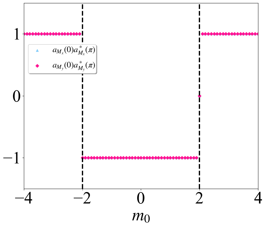
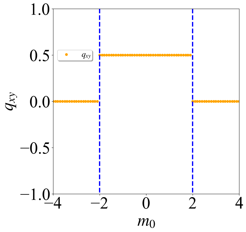
通过上面的计算可以看到,在$m_0\in(-2,2)$的区间内,$\mathcal{M}_x$和$\mathcal{M}_y$的本征值在$0$和$\pi$位置处都是相反的,那么根据
就可以确定对应的Wannier sector极化,然后通过两个不同方向的Wannier sector得到体系的电四极矩,计算结果与我们对正常态的分析是符合的。完整的代码和计算结果可以点击这里下载
参数
鉴于该网站分享的大都是学习笔记,作者水平有限,若发现有问题可以发邮件给我
- yxliphy@gmail.com
也非常欢迎喜欢分享的小伙伴投稿


欢迎关注公众号,有趣的内容也会在上面同步。 有密码的文章属于正在建设中或者没有通过验证的内容,若有需要可通过邮件联系。