这篇博客整理一下如何利用格林函数方法来计算Chern绝缘体不同边界上的边界态.
在Chern Insulator边界态及Chern数计算这篇博客中提供了计算Chern绝缘体边界态的程序,但是因为那个方法中是在一个cylinder上进行计算的,所以会存在两个边界,从而也就会在能谱中看到有两个边界态,这在有时候的研究中是不太方便的,这里就像通过格林函数的方法,计算一个半无限大的系统,因为只存在一个边界,所以对于Chern绝缘体来说此时就可以得到只有一个边界态的能谱图,而且还可以分别计算左右两端的边界态,可以发现其对应的费米速度是相反的.
计算公式
这里使用的就是Highly convergent schemes for the calculation of bulk and surface Green functions这篇文章中的计算方法,不过需要对写程序中一些具体内容进行一下说明.
当将一个动量空间中的哈密顿量沿某一个方向取开边界,另一个方向取周期边界的时候,对应的哈密顿量矩阵为
\[H=\left[\begin{array}{ccccc}H_{00}&H_{01}&0&0&0\\ H_{10}&H_{11}&H_{12}&0&0\\0&H_{21}&H_{22}&H_{23}&0\\ 0&0&H_{32}&H_{33}&\cdots\\ 0&0&0&\cdots&\cdots \end{array}\right]\]因为哈密顿量是厄米的,所以就会有$H_{01}=H_{i,i+1}=H^\dagger_{i+1,i},H_{00}=H_{ii}=H_{i+1.i+1}$.
想要得到格林函数
\[(\omega-H)G=I\]可以通过下面的迭代方程进行
\[\begin{equation}\begin{aligned}\alpha_i&=\alpha_{i-1}(\omega-\epsilon_{i-1})^{-1}\alpha_{i-1}\\ \beta_i&=\beta_{i-1}(\omega-\epsilon_{i-1})^{-1}\beta_{i-1}\\ \epsilon_i&=\epsilon_{i-1}+\alpha_{i-1}(\omega-\epsilon_{i-1})^{-1}\beta_{i-1}+\beta_{i-1}(\omega-\epsilon_{i-1})^{-1}\alpha_{i-1}\\ \epsilon^s_i&=\epsilon^s_{i-1}+\alpha_{i-1}(\omega-\epsilon_{i-1})^{-1}\beta_{i-1} \end{aligned}\end{equation}\]初始值的选择为$\epsilon_0=H_{00},\alpha_0=H_{01},\beta_0=H^\dagger_{01}$.通过一定的迭代循环之后就可以得到对应的$\epsilon^s,\epsilon$.利用这两个得到的值就可以计算哈密顿量对应的边界态,
\[A(k,\omega)=-\text{Im}[\log(\epsilon^s)]/\pi\]上面计算的是一端的边界态,如果想计算另外一端的边界态,需要对迭代进行修改
\[\epsilon^s_i=\epsilon^s_{i-1}+\beta_{i-1}(\omega-\epsilon_{i-1})^{-1}\alpha_{i-1}\]即可,计算结果如下
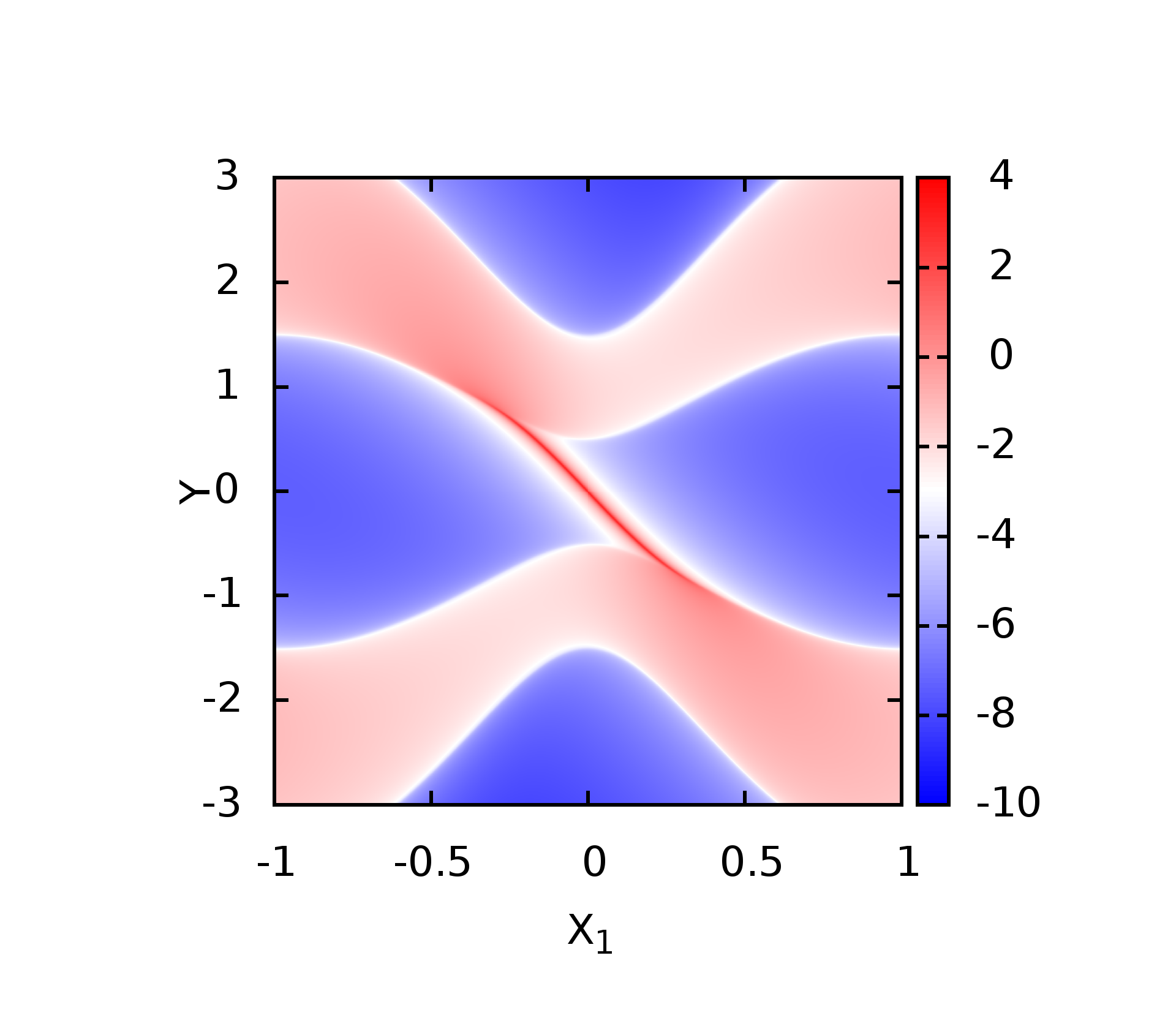
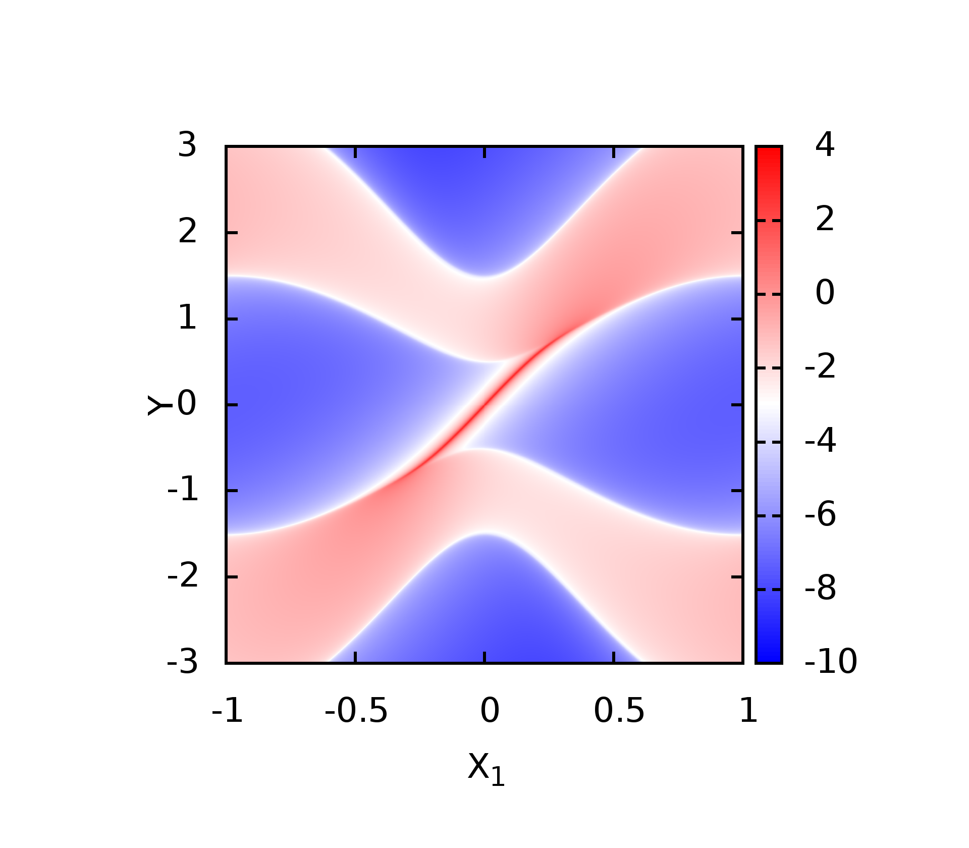

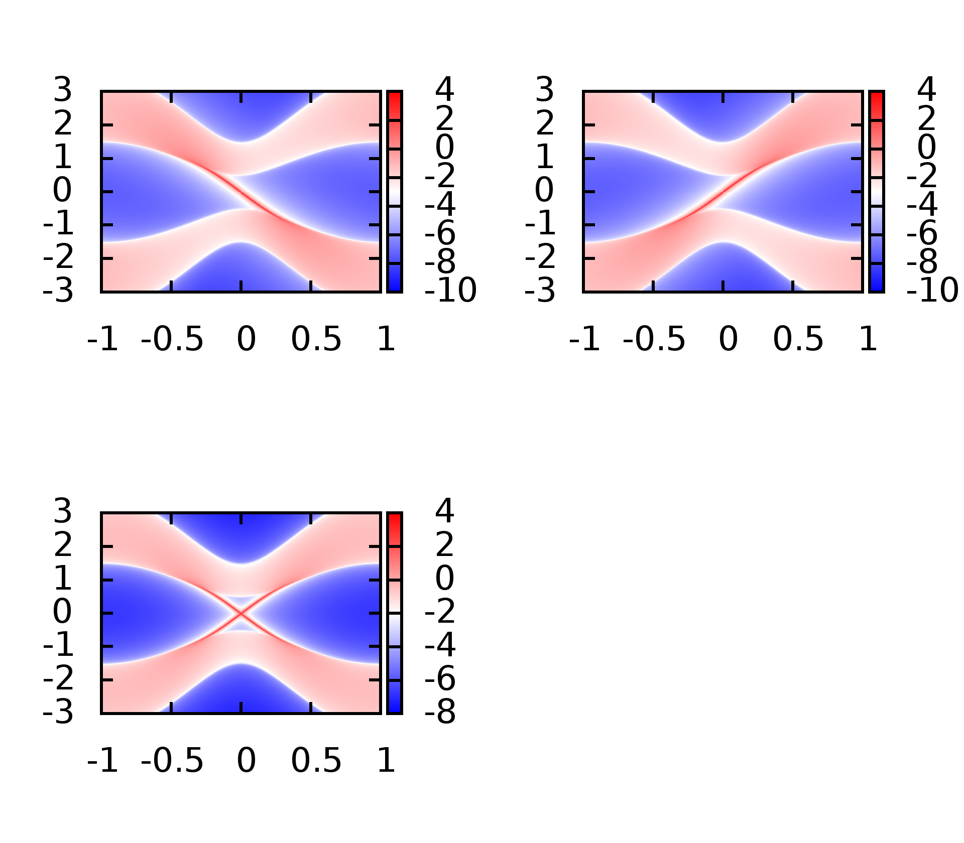
这里的第三张是将两个边界态同时计算的结果.
代码
Julia
using LinearAlgebra,DelimitedFiles,PyPlot
#---------------------------------------------------
function Pauli()
    hn = 4
    g1 = zeros(ComplexF64,hn,hn)
    g2 = zeros(ComplexF64,hn,hn)
    g3 = zeros(ComplexF64,hn,hn)
    #------
    g1[1,1] = 1
    g1[2,2] = -1
    #--------
    g2[1,2] = 1
    g2[2,1] = 1
    #---------
    g3[1,2] = -1im
    g3[2,1] = 1im
    return g1,g2,g3
end
# ========================================================
function matset(ky::Float64)
    hn::Int64 = 2
    H00 = zeros(ComplexF64,hn,hn)
    H01 = zeros(ComplexF64,hn,hn)
    g1 = zeros(ComplexF64,hn,hn)
    g2 = zeros(ComplexF64,hn,hn)
    g3 = zeros(ComplexF64,hn,hn)
    #--------------------
    m0::Float64 = 1.5
    tx::Float64 = 1.0
    ty::Float64 = 1.0
    ax::Float64 = 1.0
    ay::Float64 = 1.0
    g1,g2,g3 = Pauli()
    #--------------------
    for m in 1:hn
        for l in 1:hn
            H00[m,l] = (m0-ty*cos(ky))*g1[m,l] + ay*sin(ky)*g3[m,l]

            H01[m,l] = (-tx*g1[m,l] - 1im*ax*g2[m,l])/2
        end
    end
    #------
    return H00,H01
end
# ====================================================================================
function gf(omg::Float64,ky::Float64)
    hn::Int64 = 2
    iter::Int64 = 0
    itermax::Int64 = 100
    eta::Float64 = 0.01
    omegac::ComplexF64 = 0.0
    accuarrcy::Float64 = 1E-7
    erracc::Float64 = 0.0
    epsilon0 = zeros(ComplexF64,hn,hn)
    epsilon0s_1 = zeros(ComplexF64,hn,hn)
    epsilon0s_2 = zeros(ComplexF64,hn,hn)
    epsiloni = zeros(ComplexF64,hn,hn)
    epsilonis_1 = zeros(ComplexF64,hn,hn)
    epsilonis_2 = zeros(ComplexF64,hn,hn)
    alpha0 = zeros(ComplexF64,hn,hn)
    alphai = zeros(ComplexF64,hn,hn)
    beta0 = zeros(ComplexF64,hn,hn)
    betai = zeros(ComplexF64,hn,hn)
    H00 = zeros(ComplexF64,hn,hn)
    H01 = zeros(ComplexF64,hn,hn)
    unit = zeros(ComplexF64,hn,hn)
    GLL = zeros(ComplexF64,hn,hn)
    GRR = zeros(ComplexF64,hn,hn)
    GBulk = zeros(ComplexF64,hn,hn)
    #------------------------------------------
    omegac = omg + 1im*eta
    H00,H01 = matset(ky)
    epsilon0s_1 = H00
    epsilon0s_2 = H00
    epsilon0 = H00
    alpha0 = H01
    beta0 = conj(transpose(H01))
    #-------------------------------------
    for i in 1:hn
        unit[i,i] = 1
    end
    #--------------------------------------------
    for iter in 1:itermax
        epsilonis_1 = epsilon0s_1 + alpha0*inv(omegac*unit - epsilon0)*beta0
        epsilonis_2 = epsilon0s_2 + beta0*inv(omegac*unit - epsilon0)*alpha0

        epsiloni = epsilon0 + alpha0*inv(omegac*unit - epsilon0)*beta0 + beta0*inv(omegac*unit - epsilon0)*alpha0
        alphai = alpha0*inv(omegac*unit - epsilon0)*alpha0
        betai = beta0*inv(omegac*unit - epsilon0)*beta0

        epsilon0s_1 = epsilonis_1
        epsilon0s_2 = epsilonis_2

        epsilon0 = epsiloni
        alpha0 = alphai
        beta0 = betai
        erracc = abs(sum(alphai))
        if erracc < accuarrcy
            break
        end
    end
    # GLL = inv(omegac*unit - epsilon0s)
    # GBulk = inv(omegac*unit - epsilon0)
    GLL = epsilon0s_1
    GRR = epsilon0s_2
    GBulk = epsilon0
    return GLL,GRR,GBulk
end
# ==========================================================
function main()
    hn::Int64 = 2
    dk::Float64 = 0.01
    domg::Float64 = 0.01
    ky::Float64 = 0.0
    omg::Float64 = 0.0
    GLL = zeros(ComplexF64,hn,hn)
    GRR = zeros(ComplexF64,hn,hn)
    GBulk = zeros(ComplexF64,hn,hn)
    f1 = open("test.dat","w")
    for ky in -pi:dk:pi
        for omg in -3:domg:3
            GLL,GRR,GBulk = gf(omg,ky)
            re1 = log(-imag(sum(GLL))/pi)
            re2 = log(-imag(sum(GRR))/pi)
            re3 = log(-imag(sum(GBulk))/pi)
            writedlm(f1,[ky/pi omg re1 re2 re3],"\t")
        end
        writedlm(f1,"\n")
    end
    close(f1)
end
# =========================================================
# @time main()
main()
- 首先通过julia计算得到对应的数据
 program main
    implicit none
    integer m1,m2,m3
    call main1()
    stop
    end program
!=======================================================
    subroutine main1()
    ! 读取不明行数的文件
    implicit none
    integer count,stat
    real h1,h2,h3,h4,h5,h22
    h1 = 0
    h2 = 0
    h3 = 0
    h22 = 0
    open(1,file = "test.dat")
    open(2,file = "test-format.dat")
    count = 0
    do while (.true.)
        count = count + 1
        h22 = h1
        read(1,*,iostat = STAT)h1,h2,h3,h4,h5
        if(h22.ne.h1)write(2,*)""  ! 在这里加空行是为了gnuplot绘制密度图
        write(2,999)h1,h2,h3,h4,h5   ! 数据格式化
        if(stat .ne. 0) exit ! 当这个参数不为零的时候,证明读取到文件结尾
    end do
    ! write(*,*)h1,h2,h3
    ! write(*,*)count
    close(1)
    close(2)
999 format(10f11.6)
    return
    end subroutine main1
- 接下来通过fortran来将数据进行格式化之后,准备作图
set encoding iso_8859_1
#set terminal  postscript enhanced color
#set output 'arc_r.eps'
#set terminal pngcairo truecolor enhanced  font ",50" size 1920, 1680
set terminal png truecolor enhanced font ",50" size 1920, 1680
set output 'Chern-3.png'
#set palette defined ( -10 "#194eff", 0 "white", 10 "red" )
set palette defined ( -10 "blue", 0 "white", 10 "red" )
#set palette rgbformulae 33,13,10
unset ztics
unset key
set pm3d
set border lw 6
set size ratio 1
set view map
set xtics
set ytics
#set xlabel "K_1 (1/{\305})"
set xlabel "X_1"
#set ylabel "K_2 (1/{\305})"
set ylabel "Y"
set ylabel offset 1, 0
set colorbox
set xrange [-1:1]
set yrange [-3:3]
set pm3d interpolate 4,4
#splot 'wavenorm.dat' u 1:2:3 w pm3d
#splot 'wavenorm.dat' u 1:2:3 w pm3d
splot 'test-format.dat' u 1:2:5 w pm3d
- 最后利用gnuplot进行图形绘制即可
Fortran
同样可以利用Fortran来进行计算
    module pub
    implicit none
    integer N,iternum,hn
    real err,eta,dk,domg
    parameter( hn = 2, N = hn,iternum = 200,err = 1e-16,eta = 0.01,dk = 0.01,domg = dk)
    real,parameter::pi = 3.1415926535
    complex,parameter::im = (0.,1.0)
    complex ones(N,N),GLL(N,N),GRR(N,N),GB(N,N)
    complex H00(N,N)  ! diagonal elementery
    complex H01(N,N)  ! off-diag elementery
    complex g1(hn,hn),g2(hn,hn),g3(hn,hn)
    !---------------------------------------------
    real m0,mu
    real tx,ty
    real ax,ay
    end module pub
!==================================================================
    program main
    use pub
    !======parameter value setting =====
    m0 = 1.5
    tx = 1.0
    ty = 1.0
    ax = 1.0
    ay = 1.0
    call surfstat()
    stop
    end program main
!============================================================================================
    subroutine surfstat()
    ! surfstat calculates surface state using green's function method---J.Phys.F.Met.Phys.15(1985)851-858
    ! 利用已经求得的格林函数来计算对应的态密度
    use pub
    implicit none
    real kx,omg,re1,re2,re3
    real t_start,t_end
    integer i1
    open(20,file="dos.dat")
    call cpu_time(t_start)
    !------------------------------------------
    do kx = -pi,pi,dk
        call matset(kx)
        do omg = -3,3,domg
            call itera(omg,kx)
            re1 = log(abs(sum(aimag(GLL))))
            re2 = log(abs(sum(aimag(GRR))))
            re3 = log(abs(sum(aimag(GB))))
            write(20,999)kx/pi,omg,re1,re2,re3
        end do
        write(20,*)" "
    end do
    !------------------------------------------
    call cpu_time(t_end)
    close(20)
    write(*,*)"Timing const is: ",t_end - t_start
999 format(30f16.12)
    return
    end subroutine surfstat
!=================================================================
    subroutine itera(omega,ky)
    use pub
    real omega,real_temp,ky
    integer iter
    complex omegac
    complex g0dem(N,N), g0(N,N) ! Green's Function
    complex epsiloni(N,N),epsilons(N,N),epsilons_t(N,N),alphai(N,N),betai(N,N)   ! 迭代过程变量
    complex GLLdem(N,N),GRRdem(N,N),GBdem(N,N),mat1(N,N),mat2(N,N)
    !----------------------------
    call matset(ky)
    epsiloni = H00
    epsilons = H00
    epsilons_t = H00
    alphai = H01
    betai  = conjg(transpose(H01))
    omegac = omega + eta*im
    !----------------------------------
    do iter = 1, iternum

        g0dem = omegac*ones - epsiloni  !  Green's Function
        call inv(g0dem, g0)

        mat1 = matmul(alphai, g0)

        mat2 = matmul(betai, g0)

        g0 = matmul(mat1,betai)

        epsiloni = epsiloni + g0

        epsilons = epsilons + g0

        g0 = matmul(mat2,alphai)

        epsiloni = epsiloni + g0

        epsilons_t = epsilons_t + g0

        g0 = matmul(mat1, alphai)
        alphai = g0

        g0 = matmul(mat2, betai)
        betai = g0

        real_temp = sum(abs(alphai))
        if (real_temp .le. err)then
            exit
        end if

     end do ! end of iteration

     ! calculate surface green's function
     GLLdem = omegac*ones- epsilons
     call inv(GLLdem, GLL)
    !  GLL = epsilons


     GRRdem = omegac*ones- epsilons_t
     call inv(GRRdem, GRR)
    !  GRR = epsilons_t

     GBdem = omegac*ones- epsiloni
     call inv(GBdem, GB)
    !  GB = epsiloni
    end subroutine itera
!================================================================
    subroutine matset(ky)
    ! 构建哈密顿量
    use pub
    real ky
    integer m,l
    call Pauli()
    do m = 1,hn
        do l = 1,hn
            H00(m,l) = (m0-ty*cos(ky))*g1(m,l) + ay*sin(ky)*g3(m,l)

            H01(m,l) = (-tx*g1(m,l) - im*ax*g2(m,l))/2
        end do
    end do
    !----------------------
    !  初始化单位矩阵
    do ix = 1,N
        ones(ix,ix) = 1.0
    end do
    return
    end subroutine matset
!=======================矩阵求逆====================================
    subroutine inv(matin,matout)
    use pub
    complex,intent(in) :: matin(N,N)  ! N is dimension of matrix which can be readed from pub model (use pub)
    complex:: matout(size(matin,1),size(matin,2))
    real:: work2(size(matin,1))            ! work2 array for LAPACK
    integer::ipiv(size(matin,1))     ! pivot indices
    integer info  ! inv solution information
    ! Store matin in matout to prevent it from being overwritten by LAPACK
    matout = matin
    ! SGETRF computes an LU factorization of a general M-by-N matrix A
    ! using partial pivoting with row interchanges.
    call CGETRF(N,N,matout,N,ipiv,info)
    if (info.ne.0) stop 'Matrix is numerically singular!'
    ! SGETRI computes the inverse of a matrix using the LU factorization
    ! computed by SGETRF.
    call CGETRI(N,matout,N,ipiv,work2,N,info)
    if (info.ne.0) stop 'Matrix inversion failed!'
    return
    end subroutine inv
!====================================================
    subroutine Pauli()
    use pub
    !----------
    g1(1,1) = 1
    g1(2,2) = -1
    !----------
    g2(1,2) = 1
    g2(2,1) = 1
    !----------
    g3(1,2) = -im
    g3(2,1) = im
    return
    end subroutine Pauli
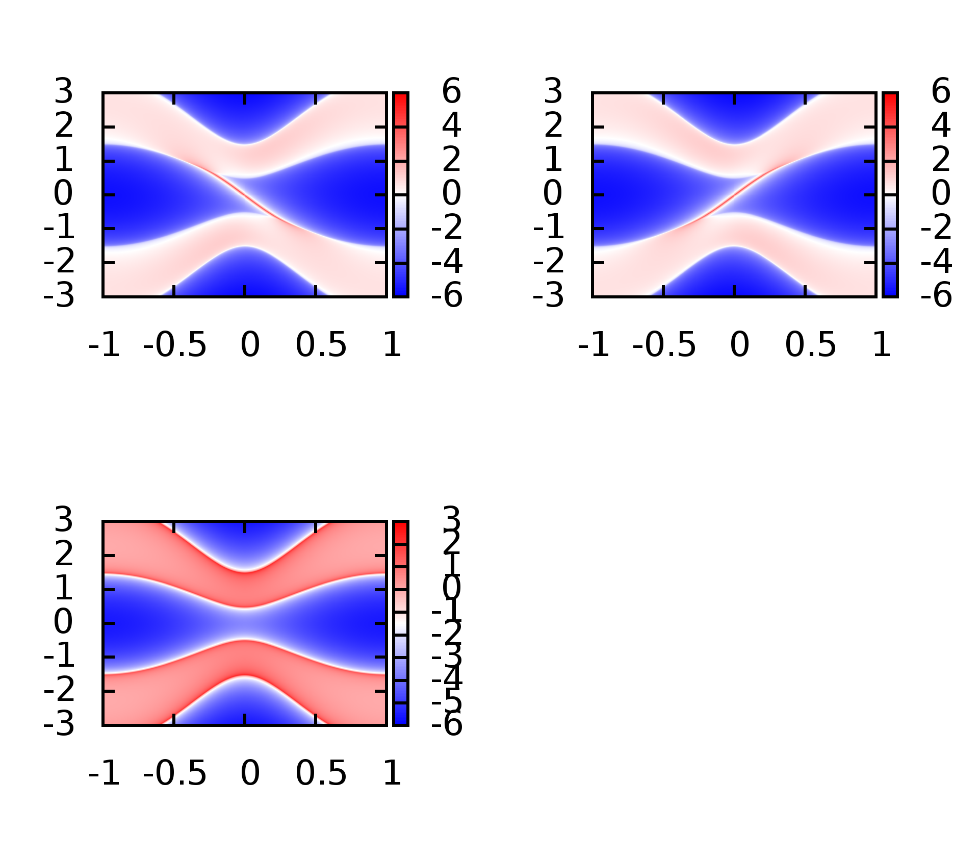
此时可以同时计算出左边界,有边界以及体态的能带.
补充
上面是将三张分开绘制的,利用的分别是数据的第三,第四,第五列,这里将三个结果绘制到统一张图上
set encoding iso_8859_1
#set terminal  postscript enhanced color
#set output 'arc_r.eps'
#set terminal pngcairo truecolor enhanced  font ",50" size 1920, 1680
set terminal png truecolor enhanced font ",50" size 1920, 1680
set output 'Chern.png'
#set size 2, 1
#set palette defined ( -10 "#194eff", 0 "white", 10 "red" )
set palette defined ( -10 "blue", 0 "white", 10 "red" )
#set palette rgbformulae 33,13,10
set multiplot layout 2,2
unset ztics
unset key
set pm3d
set border lw 6
#set size ratio 1
set view map
#set xtics
#set ytics
#set xlabel "K_1 (1/{\305})"
#set xlabel "X_1"
#set ylabel "K_2 (1/{\305})"
#set ylabel "Y"
#set ylabel offset 1, 0
set colorbox
set xrange [-1:1]
set yrange [-3:3]
set pm3d interpolate 4,4
#splot 'wavenorm.dat' u 1:2:3 w pm3d
#splot 'wavenorm.dat' u 1:2:3 w pm3d
splot 'test-format.dat' u 1:2:3 w pm3d
splot 'test-format.dat' u 1:2:4 w pm3d
splot 'test-format.dat' u 1:2:5 w pm3d
Python Version
最近搞科研,发现许多函数还是使用python比较好,借用其比较好的生态,想要实现某些功能不需要自己去写相对应的函数
import numpy as np
import matplotlib.pyplot as plt
import os
import time
import seaborn as sns

def Pauli():
    s0 = np.array([[1,0],[0,1]])
    sx = np.array([[0,1],[1,0]])
    sy = np.array([[0,-1j],[1j,0]])
    sz = np.array([[1,0],[0,-1]])
    return s0,sx,sy,sz
#------------------------------------------------
def hamset(ki):
    m0 = 1.5
    tx = 1.0
    ty = 1.0
    ax = 1.0
    ay = 1.0
    s0,sx,sy,sz = Pauli()
    H00 = np.zeros((2,2),np.complex128)
    H01 = np.zeros((2,2),np.complex128)
    for i0 in range(2):
        for i1 in range(2):
            H00[i0,i1] = (m0 - tx*np.cos(ki))*sz[i0,i1] + ax*np.sin(ki)*sx[i0,i1]
            H01[i0,i1] = -ty/2.0*sz[i0,i1] + ay/(2.0*1j)*sy[i0,i1]
    return H00,H01
# -----------------------------------------------------------------------
def Iteration(omega,ki):
    err = 1e-16
    eta = 0.01
    iternum = 200
    H00 = np.zeros((2,2),np.complex128)
    H01 = np.zeros((2,2),np.complex128)
    H00,H01 = hamset(ki)
    epsiloni = H00
    epsilons = H00
    epsilons_t = H00
    alphai = H01
    betai = H01.T.conjugate() # 转置共轭
    omegac = omega + eta*1j
    s0,sx,sy,sz = Pauli()
    for i0 in range(iternum):
        g0dem = omegac*s0 - epsiloni

        g0 = np.linalg.inv(g0dem)

        mat1 = np.dot(alphai,g0)

        mat2 = np.dot(betai,g0)

        g0 = np.dot(mat1,betai)

        epsiloni = epsiloni + g0

        epsilons = epsilons + g0

        g0 = np.dot(mat2,alphai)

        epsiloni = epsiloni + g0

        epsilons_t = epsilons_t + g0

        g0 = np.dot(mat1, alphai)

        alphai = g0

        g0 = np.dot(mat2,betai)

        betai = g0

        real_temp = np.sum(np.concatenate(np.abs(alphai)))

        if (real_temp < err):
            break

    GLLdem = omegac*s0 - epsilons
    GLL = np.linalg.inv(GLLdem)
    #  GLL = epsilons
    GLL =  np.sum(np.concatenate(np.abs(GLL)))


    GRRdem = omegac*s0 - epsilons_t
    GRR = np.linalg.inv(GRRdem)
    GRR =  np.sum(np.concatenate(np.abs(GRR)))
    #  GRR = epsilons_t

    GBdem = omegac*s0 - epsiloni
    GB = np.linalg.inv(GBdem)
    GB =  np.sum(np.concatenate(np.abs(GB)))
    #  GB = epsiloni

    return GLL,GRR,GB
#------------------------------------------------------------
def surface():
    nx = 100
    max_omg = 1.5
    re = np.zeros((len(range(-nx,nx))**2,5))
    con = 0
    ix = -1
    iy = -1
    GLL = np.zeros((len(range(-nx,nx)),len(range(-nx,nx))))
    GRR = np.zeros((len(range(-nx,nx)),len(range(-nx,nx))))
    GB = np.zeros((len(range(-nx,nx)),len(range(-nx,nx))))
    for i0 in range(-nx,nx):
        kx = np.pi*i0/nx
        for i1 in range(-nx,nx):
            omg = max_omg*i1/nx
            re1,re2,re3 = Iteration(omg,kx)
            re[con,0] = kx
            re[con,1] = omg
            re[con,2] = re1
            re[con,3] = re2
            re[con,4] = re3

            GLL[iy,ix] = np.log(re1)
            GRR[iy,ix] = np.log(re2)
            GB[iy,ix] = np.log(re3)
            con += 1
            iy += 1
        ix += 1
        iy = 0
#     np.savetxt("GLL.dat", [kilist,re1list], fmt="%15.10f")
#     np.savetxt("GRR.dat", [kilist,re1list], fmt="%15.10f")
#     np.savetxt("GB.dat", [kilist,re1list], fmt="%15.10f")
    np.savetxt("density.dat",re , fmt="%15.10f")
    return GLL,GRR,GB
#-----------------------------------------------------------------------
def main():
    os.chdir(os.getcwd())
    tstart = time.time()
    GLL,GRR,GB = surface()
    tend = time.time()
    #print(tend - tstart)
    # 绘图
    sns.set()
    ax = sns.heatmap(GB)
    plt.show()
#-----------------------------------------------------------------------
if __name__ == '__main__':
    main()
这里最终计算的结果肯定是相同的,只不过绘图的时候给出的横纵坐标我没有去设置,这个具体使用的时候,到后面再去慢慢调整。
参考
公众号
相关内容均会在公众号进行同步,若对该Blog感兴趣,欢迎关注微信公众号。

|
yxli406@gmail.com |