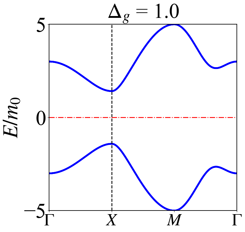
通常为了看是否发生拓扑相变需要关注参数演化的时候能带是否发生了闭合,而且也只需要关注布里渊区高对称路径上的能带演化即可,这里就整理了自己的一个小程序,方便自己在研究问题的时候直接拿来就使用。
2D suqare lattice
写程序的想法就是直接给出动量空间中的哈密顿量,通过对角化的方式得到本征值,将这一过程沿着高对称路径进行即可。
from cmath import pi
import numpy as np
import matplotlib.pyplot as plt
from matplotlib import rcParams
import os
config = {
"font.size": 40,
"mathtext.fontset":'stix',
"font.serif": ['SimSun'],
}
rcParams.update(config) # Latex 字体设置
#-------------------------------------------------------------
def Pauli():
    s0 = np.array([[1, 0], [0, 1]])
    sx = np.array([[0, 1], [1, 0]])
    sy = np.array([[0, -1j], [1j, 0]])
    sz = np.array([[1, 0], [0, -1]])
    return s0, sx, sy, sz
# --------------------------------------------------------------
def hamset(kx, ky, dg):
    hn = 8
    s0 = np.zeros([2, 2], dtype=complex)
    sx = np.zeros([2, 2], dtype=complex)
    sy = np.zeros([2, 2], dtype=complex)
    sz = np.zeros([2, 2], dtype=complex)
    ham = np.zeros([hn, hn], dtype=complex)
    m0 = 1.0
    tx = 2.0
    ty = 2.0
    txy = 0.0
    ax = 2.0
    ay = 2.0
    d0 = 0.
    dx = 0.5
    dy = -dx
    # dg = 0.5
    s0, sx, sy, sz = Pauli()
    ham = (m0 - tx * np.cos(kx) - ty * np.cos(ky) - 2 * txy * np.cos(kx) * np.cos(ky)) * np.kron(np.kron(s0, sz),sz)\
            + ax * np.sin(kx) * np.kron(np.kron(sz, sx), s0)\
            + ay * np.sin(ky) * np.kron(np.kron(s0, sy), sz)\
            + (d0 + dx * np.cos(kx) + dy * np.cos(ky)) * np.kron(np.kron(sy, s0), sy)\
            + (dg*(np.cos(kx) - np.cos(ky))*np.sin(kx)*np.sin(ky)) * np.kron(np.kron(sy, s0), sx)
    vals,vecs = np.linalg.eigh(ham)
    return vals
#-----------------------------------------------------------
def HSP(hx):
    kxlist = np.linspace(0,np.pi,100)
    relist1 = []
    x0 = []
    for kx in kxlist:
        x0.append(kx/np.pi)
        relist1.append(hamset(kx,0,hx))
    for ky in kxlist:
        x0.append(ky/np.pi + 1)
        relist1.append(hamset(np.pi,ky,hx))
    for k in kxlist:
        x0.append(k/np.pi + 2)
        relist1.append(hamset(np.pi - k,np.pi - k,hx))

    plt.figure(figsize=(8,8))
    # plt.plot(x0,y01,c = "blue" ,lw = 4,label = r"$\tilde{M}^+_I\times \tilde{M}^+_{II}$")
    # plt.plot(x0,y02,c = "red" ,lw = 4,label = r"$\tilde{M}^-_I\times \tilde{M}^-_{II}$")
    plt.plot(x0,relist1,c = "blue" ,lw = 4)
    # plt.plot(x0,relist2,c = "blue" ,lw = 4)
    # plt.plot(x0,relist3,c = "blue" ,lw = 4)
    # plt.plot(x0,relist4,c = "blue" ,lw = 4)
    # plt.plot(x0,y02,c = "red" ,lw = 4,label = r"$\tilde{M}^-$")
    font2 = {'family': 'Times New Roman',
             'weight': 'normal',
             'size': 50,
             }
    x0min = np.min(x0)
    x0max = np.max(x0)
    y0max = np.max(relist1)
    # y0max = 5
    # plt.ylim(yaxmin,yaxman + 0.25)
    # plt.text(pp1 - 0.2,-0.8,r"$0.23\pi$",color = "green")
    # plt.text(pp2 ,-0.8,r"$0.27\pi$",color = "green")
    plt.vlines(1,ymin = -y0max,ymax = y0max,lw = 2,colors = "black",ls = "--")
    # plt.vlines(2,ymin = -y0max,ymax = y0max,lw = 2,colors = "black",ls = "--")
    plt.hlines(0,xmin = x0min,xmax = x0max,lw = 2,colors = "red",ls = "-.")
    xtic = [0,1,2,3]
    xticlab = ["$\Gamma$",r"$X$","$M$","$\Gamma$"]
    plt.xticks(xtic,list(xticlab),fontproperties='Times New Roman', size = 40)
    plt.yticks([-5,0,5],fontproperties='Times New Roman', size = 50)
    plt.ylabel("$E/m_0$", font2)
    plt.xlim(x0min,x0max)
    plt.ylim(-y0max,y0max)
    tit = "$\Delta_g$ = " + str(hx)
    plt.title(tit,font2)
    # plt.legend(loc = 'upper right', ncol = 1, shadow = True, fancybox = True, prop = font1, markerscale = 0.5) # 图例
    # ax1.patch.set_facecolor("lightblue")    # 设置 ax1 区域背景颜⾊
    # ax1.patch.set_alpha(0.5)    # 设置 ax1 区域背景颜⾊透明度
    # plt.show()
    ax = plt.gca()
    # ax.patch.set_facecolor("lightblue")    # 设置 ax1 区域背景颜⾊
    # ax.patch.set_alpha(0.5)    # 设置 ax1 区域背景颜⾊透明度
    ax.spines["bottom"].set_linewidth(1.5)
    ax.spines["left"].set_linewidth(1.5)
    ax.spines["right"].set_linewidth(1.5)
    ax.spines["top"].set_linewidth(1.5)
    picname = "hsp2-" + str(format(hx,".2f")) + ".png"
    plt.savefig(picname, dpi = 100, bbox_inches = 'tight')
    plt.close()
    # plt.show()
#----------------------------------------------------------------
if __name__=="__main__":
    HSP(1.0)
公众号
相关内容均会在公众号进行同步,若对该Blog感兴趣,欢迎关注微信公众号。

|
yxli406@gmail.com |