超导磁电效应

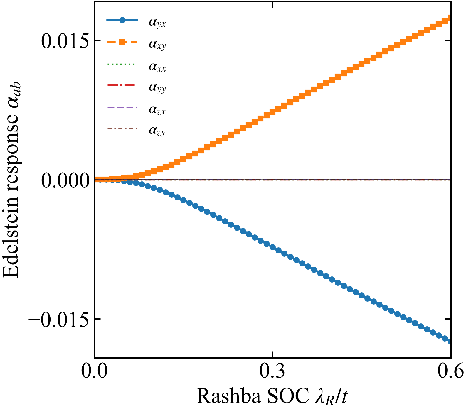
超导线性磁电效应，也叫超导Edelstein效应，描述的是超流驱动产生自旋磁化。超流可以用 Cooper pair 的有限动量 $\mathbf q$ 表示。对于小 $\mathbf q$，自旋磁化可以展开为

$M_a(\mathbf q) = M_a^{(0)} + \delta M_a^{(1)} + O(q^2),$

其中线性磁电效应定义为

${ \delta M_a^{(1)}=\alpha_{ab}q_b . }$

若进一步用超流密度 $\mathbf J_s$ 表示，由于$J_{s,b}=\nu_s q_b$，也可以写成

$\delta M_a^{(1)} = \frac{\alpha_{ab}}{\nu_s}J_{s,b}.$

考虑一般正常态 Bloch哈密顿量$H_{\mathbf k}$，它可以包含轨道、自旋、子格等内部自由度。超导配对矩阵记为$\hat\Delta_{\mathbf k}$，若超导序参量携带空间相位$\Delta(\mathbf r)=\Delta_0 e^{i\mathbf q\cdot \mathbf r}$，则 Cooper对的总动量为 $\mathbf q$。配对的两个电子动量可以写成

$\mathbf k+\frac{\mathbf q}{2}, \qquad -\mathbf k+\frac{\mathbf q}{2}.$

于是定义 Nambu 基底

$\Psi_{\mathbf k,\mathbf q} = \begin{pmatrix} c_{\mathbf k+\mathbf q/2}\\ c^\dagger_{-\mathbf k+\mathbf q/2} \end{pmatrix}.$

在显式自旋基底下，可以写为

$\Psi_{\mathbf k,\mathbf q} = \left( c_{\mathbf k+\mathbf q/2,\uparrow}, c_{\mathbf k+\mathbf q/2,\downarrow}, c^\dagger_{-\mathbf k+\mathbf q/2,\uparrow}, c^\dagger_{-\mathbf k+\mathbf q/2,\downarrow} \right)^T .$

有限 $\mathbf q$ 的 BdG Hamiltonian 为

${ \mathcal H_{\rm BdG}(\mathbf k,\mathbf q) = \begin{pmatrix} H_{\mathbf k+\mathbf q/2} & \hat\Delta_{\mathbf k}\\ \hat\Delta_{\mathbf k}^\dagger & -H^*_{-\mathbf k+\mathbf q/2} \end{pmatrix}. }$

这里暂时假设 $\hat\Delta_{\mathbf k}$ 不显式依赖 $\mathbf q$。这个近似适用于弱超流，也就是 $\mathbf q$ 足够小的情况。

磁化的热力学定义

为了计算自旋磁化，引入一个辅助 Zeeman 场 $\mathbf h$。电子的 Zeeman 耦合为

$-\frac{g_s\mu_B}{2}\mathbf h\cdot \mathbf s,$

其中 $s_a$ 是 Pauli 矩阵，真正的自旋算符是 $s_a/2$。在 Nambu 空间中，相应的广义自旋矩阵定义为

${\color{blue} \eta_a = \begin{pmatrix} s_a & 0\\ 0 & -s_a^* \end{pmatrix}. }$

这里空穴块前面的负号来自粒子—-空穴结构。含辅助 Zeeman 场的格林函数写成

$G^{-1}(\mathbf k,\mathbf q,\mathbf h,i\omega_n) = G^{-1}(\mathbf k,\mathbf q,i\omega_n) + \Sigma(\mathbf h),\quad \Sigma(\mathbf h) = \frac{g_s\mu_B}{2} \mathbf h\cdot \boldsymbol{\eta}.$

Gor’kov 格林函数为

$G(\mathbf k,\mathbf q,i\omega_n) = \left[ i\omega_n-\mathcal H_{\rm BdG}(\mathbf k,\mathbf q) \right]^{-1}.$

辅助场 $\mathbf h$ 最后要取零。磁化由配分函数对 $\mathbf h$ 求导得到

$M_a = -\frac{1}{\beta} \frac{\partial \log Z(\mathbf h)} {\partial h_a} \bigg|_{\mathbf h=0}.$

由于 Nambu 表象中有一半的 double counting，配分函数中出现因子 $1/2$。对 $\mathrm{Tr}\log G^{-1}$ 求导，使用

$\frac{\partial}{\partial h_a} \mathrm{Tr}\log G^{-1} = \mathrm{Tr} \left[ G \frac{\partial G^{-1}}{\partial h_a} \right],\qquad \frac{\partial G^{-1}}{\partial h_a} = \frac{g_s\mu_B}{2}\eta_a,$

得到

${\color{blue} M_a(\mathbf q) = -\frac{g_s\mu_B}{4\beta} \sum_{\mathbf k,n} \mathrm{Tr} \left[ G(\mathbf k,\mathbf q,i\omega_n)\eta_a \right]. }\label{eq:m2}$

现在对$\mathcal H_{\rm BdG}(\mathbf k,\mathbf q)$在 $\mathbf q=0$ 附近展开，首先定义没有超流态的 BdG 哈密顿量

$\mathcal H_0(\mathbf k) \equiv \mathcal H_{\rm BdG}(\mathbf k,\mathbf q=0) = \begin{pmatrix} H_{\mathbf k} & \hat\Delta_{\mathbf k}\\ \hat\Delta_{\mathbf k}^\dagger & -H^*_{-\mathbf k} \end{pmatrix}.$

正常态速度矩阵定义为

$V_b(\mathbf k) = \frac{\partial H_{\mathbf k}}{\partial k_b}.$

由于电子块是 $H_{\mathbf k+\mathbf q/2}$，所以一阶展开为

$H_{\mathbf k+\mathbf q/2} = H_{\mathbf k} + \frac{q_b}{2} V_b(\mathbf k) + O(q^2).$

空穴块是$-H^*_{-\mathbf k+\mathbf q/2}$，因此一阶展开为

$-H^*_{-\mathbf k+\mathbf q/2} = -H^*_{-\mathbf k} - \frac{q_b}{2} V_b^*(-\mathbf k) + O(q^2)$

所以 BdG Hamiltonian 的一阶展开可以写成

${\color{blue} \mathcal H_{\rm BdG}(\mathbf k,\mathbf q) = \mathcal H_0(\mathbf k) + \frac{q_b}{2} \hat v_b(\mathbf k) + O(q^2), }\label{eq:m1}$

其中 Nambu 空间速度矩阵为

${ \hat v_b(\mathbf k) = \begin{pmatrix} V_b(\mathbf k) & 0\\ 0 & -V_b^*(-\mathbf k) \end{pmatrix}. }$

接下来对格林函数进行展开，定义没有超流态的格林函数

$G_0(\mathbf k,i\omega_n) = \left[ i\omega_n-\mathcal H_0(\mathbf k) \right]^{-1}.$

由方程$\eqref{eq:m1}$可得

$G^{-1}(\mathbf k,\mathbf q,i\omega_n) = i\omega_n-\mathcal H_{\rm BdG}(\mathbf k,\mathbf q)=G_0^{-1}-\frac{q_b}{2}\hat{v}_b(\mathbf k)$

因此

$G = \left[ G_0^{-1} - \frac{q_b}{2}\hat v_b \right]^{-1}.$

使用矩阵恒等式

$(A-B)^{-1} = A^{-1} + A^{-1}BA^{-1} + O(B^2),$

得到

${ G(\mathbf k,\mathbf q,i\omega_n) = G_0(\mathbf k,i\omega_n) + \frac{q_b}{2} G_0(\mathbf k,i\omega_n) \hat v_b(\mathbf k) G_0(\mathbf k,i\omega_n) + O(q^2). }$

将其代入方程$\eqref{eq:m2}$得到

$M_a(\mathbf q) = -\frac{g_s\mu_B}{4\beta} \sum_{\mathbf k,n} \mathrm{Tr} \left[ G_0\eta_a \right] - \frac{g_s\mu_B}{8\beta} q_b \sum_{\mathbf k,n} \mathrm{Tr} \left[ G_0\hat v_bG_0\eta_a \right] + O(q^2).$

利用迹的循环不变性

$\mathrm{Tr} \left[ G_0\hat v_bG_0\eta_a \right] = \mathrm{Tr} \left[ \eta_aG_0\hat v_bG_0 \right],$

因此

$M_a(\mathbf q) = M_a^{(0)} + \alpha_{ab}q_b + O(q^2),$

其中

$M_a^{(0)} = -\frac{g_s\mu_B}{4\beta} \sum_{\mathbf k,n} \mathrm{Tr} \left[ G_0\eta_a \right],$

而线性磁电张量为

${\color{blue} \alpha_{ab} = -\frac{g_s\mu_B}{8\beta} \sum_{\mathbf k,n} \mathrm{Tr} \left[ \eta_aG_0\hat v_bG_0 \right]. }$

这就是超导线性磁电效应的 Kubo-like格林函数形式。现在将上式改写成 BdG 能带表象，对零超流态 BdG哈密顿量对角化

${ \mathcal H_0(\mathbf k) |u_{n\mathbf k}\rangle = E_{n\mathbf k} |u_{n\mathbf k}\rangle . }$

这里 $n$ 是 BdG 能带指标。由于 BdG 哈密顿量具有粒子—-空穴对称性，能谱通常成对出现$E_{n\mathbf k}
\leftrightarrow
-E_{n,-\mathbf k}$，但是在下面的推导中，我们直接对所有 BdG 本征态求和，不需要额外区分正能和负能分支。

格林函数可以谱分解为

${ G_0(\mathbf k,i\omega_n) = \sum_l \frac{ |u_{l\mathbf k}\rangle \langle u_{l\mathbf k}| }{ i\omega_n-E_{l\mathbf k} }. }$

定义能带表象中的矩阵元

$\eta^a_{nm}(\mathbf k) = \langle u_{n\mathbf k}| \eta_a |u_{m\mathbf k}\rangle,\qquad v^b_{mn}(\mathbf k) = \langle u_{m\mathbf k}| \hat v_b(\mathbf k) |u_{n\mathbf k}\rangle.$

将格林函数的谱分解代入$\mathrm{Tr}
\left[
\eta_aG_0\hat v_bG_0
\right]$中得到

$\mathrm{Tr} \left[ \eta_aG_0\hat v_bG_0 \right] = \sum_{n,m} \frac{ \eta^a_{nm}(\mathbf k) v^b_{mn}(\mathbf k) }{ (i\omega_n-E_{m\mathbf k}) (i\omega_n-E_{n\mathbf k}) }.$

因此线性磁电张量系数为

$\alpha_{ab} = -\frac{g_s\mu_B}{8\beta} \sum_{\mathbf k} \sum_{\omega_n} \sum_{n,m} \frac{ \eta^a_{nm}(\mathbf k) v^b_{mn}(\mathbf k) }{ (i\omega_n-E_{n\mathbf k}) (i\omega_n-E_{m\mathbf k}) }.$

下面对松原频率求和，定义

$I_{nm}(\mathbf k) = \frac{1}{\beta} \sum_{\omega_n} \frac{1}{ (i\omega_n-E_{n\mathbf k}) (i\omega_n-E_{m\mathbf k}) }.$

当 $n\neq m$ 时，用部分分式分解

$\frac{1}{ (i\omega_n-E_n)(i\omega_n-E_m) } = \frac{1}{E_n-E_m} \left[ \frac{1}{i\omega_n-E_n} - \frac{1}{i\omega_n-E_m} \right].$

结合标准松原频率求和公式

$\frac{1}{\beta} \sum_{\omega_n} \frac{1}{i\omega_n-E} = -f(E),\qquad f(E)=\frac{1}{e^{\beta E}+1}$

因此

$I_{nm} = \frac{f(E_{m\mathbf k})-f(E_{n\mathbf k})} {E_{n\mathbf k}-E_{m\mathbf k}}.$

于是

$\alpha_{ab} = -\frac{g_s\mu_B}{8} \sum_{\mathbf k} \sum_{n,m} \eta^a_{nm}(\mathbf k) v^b_{mn}(\mathbf k) \frac{ f(E_{m\mathbf k})-f(E_{n\mathbf k}) }{ E_{n\mathbf k}-E_{m\mathbf k} }.$

等价的可以表示为

${ \alpha_{ab} = \frac{g_s\mu_B}{8} \sum_{\mathbf k} \sum_{n,m} \eta^a_{nm}(\mathbf k) v^b_{mn}(\mathbf k) \frac{ f(E_{n\mathbf k})-f(E_{m\mathbf k}) }{ E_{n\mathbf k}-E_{m\mathbf k} }. }$

由于 $\alpha_{ab}$ 是实物理量，通常可显式写成

${ \alpha_{ab} = \frac{g_s\mu_B}{8} \sum_{\mathbf k} \sum_{n,m} \mathrm{Re} \left[ \eta^a_{nm}(\mathbf k) v^b_{mn}(\mathbf k) \right] \frac{ f(E_{n\mathbf k})-f(E_{m\mathbf k}) }{ E_{n\mathbf k}-E_{m\mathbf k} }. }$

当$E_{n\mathbf k}=E_{m\mathbf k}$时上式需要取极限，特别是$n=m$时

$\frac{ f(E_{n\mathbf k})-f(E_{m\mathbf k}) }{ E_{n\mathbf k}-E_{m\mathbf k} } \longrightarrow f'(E_{n\mathbf k}),\qquad f'(E) = -\beta f(E)\left[1-f(E)\right].$

因此对角项为

${ \alpha_{ab}^{\rm diag} = \frac{g_s\mu_B}{8} \sum_{\mathbf k,n} f'(E_{n\mathbf k}) \eta^a_{nn}(\mathbf k) v^b_{nn}(\mathbf k). }$

注意 $f’(E)<0$。低温下，$f’(E)$ 只在 $E\approx 0$ 附近有明显贡献。因此，如果 BdG 谱完全打开能隙，那么这个对角项在 $T\to 0$ 时通常会被指数压低。

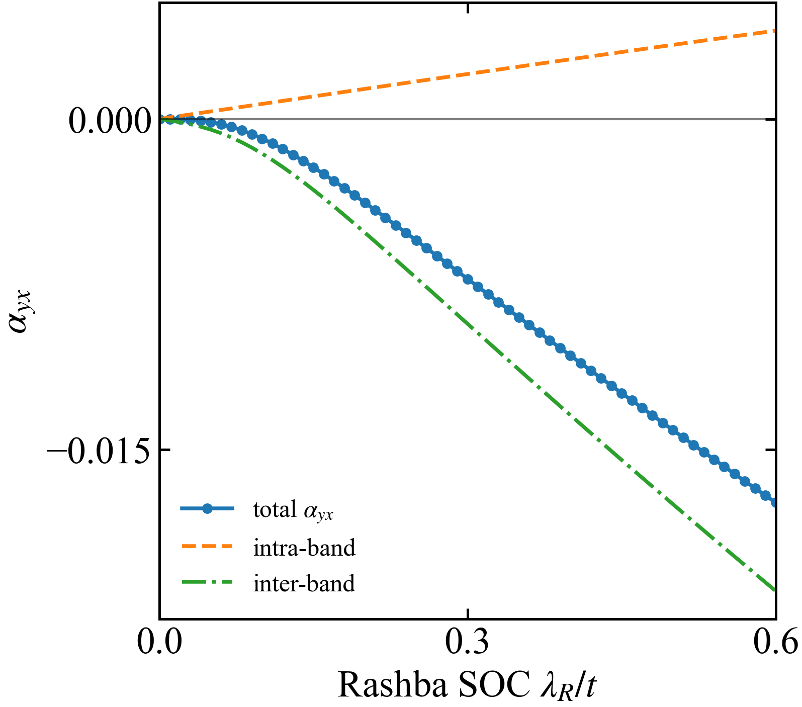
能带表象的表达式可以自然分成两部分

$\alpha_{ab} = \alpha_{ab}^{\rm intra} + \alpha_{ab}^{\rm inter}.$

对角部分，即 $n=m$，为

${ \alpha_{ab}^{\rm intra} = \frac{g_s\mu_B}{8} \sum_{\mathbf k,n} f'(E_{n\mathbf k}) \eta^a_{nn}(\mathbf k) v^b_{nn}(\mathbf k). }$

这个部分反映 BdG 准粒子能带在有限 $\mathbf q$ 下的占据变化。它类似金属正常态响应中的费米面贡献。

非对角部分，即 $n\neq m$，为

${ \alpha_{ab}^{\rm inter} = \frac{g_s\mu_B}{8} \sum_{\mathbf k} \sum_{n\neq m} \mathrm{Re} \left[ \eta^a_{nm}(\mathbf k) v^b_{mn}(\mathbf k) \right] \frac{ f(E_{n\mathbf k})-f(E_{m\mathbf k}) }{ E_{n\mathbf k}-E_{m\mathbf k} }. }$

这个部分来自不同 BdG 本征态之间的虚跃迁，类似带间极化率。也可以利用 $n,m$ 的对称性写成 $n<m$ 的形式

${ \alpha_{ab}^{\rm inter} = \frac{g_s\mu_B}{4} \sum_{\mathbf k} \sum_{n<m} \mathrm{Re} \left[ \eta^a_{nm}(\mathbf k) v^b_{mn}(\mathbf k) \right] \frac{ f(E_{n\mathbf k})-f(E_{m\mathbf k}) }{ E_{n\mathbf k}-E_{m\mathbf k} }. }$

Rashba 超导

对于二维 Rashba 超导，正常态哈密顿量可写成

$H_{\mathbf k} = \xi_{\mathbf k}s_0 + \lambda a(k_xs_y-k_ys_x),\quad \xi_{\mathbf k} = ta^2(k_x^2+k_y^2)-\mu.$

配对取常规的$s$波配对

$\hat\Delta_{\mathbf k} = \Delta_0 i s_y.$

速度矩阵为

$V_x(\mathbf k) = 2ta^2k_xs_0+\lambda a s_y,\qquad V_y(\mathbf k) = 2ta^2k_ys_0-\lambda a s_x.$

由于 Rashba SOC 使自旋和动量锁定，超流沿 $x$ 方向时，主要诱导 $y$ 方向磁化

$M_y = \alpha_{yx}q_x.$

超流沿 $y$ 方向时，主要诱导 $x$ 方向磁化

$M_x = \alpha_{xy}q_y.$

在连续旋转对称的 Rashba 系统中

$\alpha_{xy}=-\alpha_{yx}.$

因此整体上有

${ \delta \mathbf M^{(1)} \propto \hat{\mathbf z}\times \mathbf q. }$

由于

$\mathbf J_s=\nu_s\mathbf q,$

也就是

${ \delta \mathbf M^{(1)} \propto \hat{\mathbf z}\times \mathbf J_s. }$

对称性约束

线性磁电效应

$\delta M_a^{(1)} = \alpha_{ab}q_b$

对称性上要求反演对称性破缺。因为$\mathbf{q}$是极矢量，在空间反演 $P$ 下变号

$P:\quad \mathbf q\rightarrow-\mathbf q$

而磁化$\mathbf M$是轴矢量，在空间反演下不变

$P:\quad \mathbf M\rightarrow \mathbf M.$

因此如果体系有反演对称性，那么$\mathbf M\propto \mathbf q$这一线性关系被禁止$(\alpha_{ab}=0)$。但是时间反演 $T$ 本身不禁止线性磁电效应，因为

$T:\quad \mathbf M\rightarrow -\mathbf M, \qquad \mathbf q\rightarrow -\mathbf q.$

所以$\mathbf M\propto\mathbf q$在时间反演下是允许的。所以Rashba 超导可以在保持时间反演对称性的情况下存在超导Edelstein效应。

程序代码

计算代码

#!/usr/bin/env julia

# ============================================================
# Square-lattice Rashba superconductor
# Superconducting Edelstein effect
#
# MPI parallel version.
#
# Output:
#   data/rashba_lattice_edelstein_mpi.dat
#
# Tensor:
#   delta M_a = alpha_ab q_b
#
# Main Rashba Edelstein component:
#   alpha_yx : q_x -> M_y
# ============================================================

using MPI
using LinearAlgebra
using Printf
using Dates

BLAS.set_num_threads(1)

# ============================================================
# 0. MPI initialization
# ============================================================

MPI.Init()

const comm = MPI.COMM_WORLD
const rank = MPI.Comm_rank(comm)
const nprocs = MPI.Comm_size(comm)

# ============================================================
# 1. Parameters
# ============================================================

const t_hop = 1.0
const mu = -3.0
const Delta0 = 0.10
const temperature = 0.03

# k mesh
const Nk = 251

# Rashba SOC scan
const lambda_min = 0.0
const lambda_max = 0.60
const lambda_num = 61

# Constants, dimensionless units
const gs = 2.0
const muB = 1.0

# Degeneracy tolerance for K_nm
const degeneracy_eps = 1.0e-10

# Output
const data_dir = "data"
const output_file = joinpath(data_dir, "rashba_lattice_edelstein_mpi.dat")

# ============================================================
# 2. Pauli matrices
# ============================================================

const s0 = ComplexF64[
    1.0 + 0im  0.0 + 0im
    0.0 + 0im  1.0 + 0im
]

const sx = ComplexF64[
    0.0 + 0im  1.0 + 0im
    1.0 + 0im  0.0 + 0im
]

const sy = ComplexF64[
    0.0 + 0im   0.0 - 1im
    0.0 + 1im   0.0 + 0im
]

const sz = ComplexF64[
    1.0 + 0im   0.0 + 0im
    0.0 + 0im  -1.0 + 0im
]

const zero2 = zeros(ComplexF64, 2, 2)

# ============================================================
# 3. Small matrix helpers
# ============================================================

function block2x2(A::Matrix{ComplexF64}, B::Matrix{ComplexF64},
                  C::Matrix{ComplexF64}, D::Matrix{ComplexF64})
    M = zeros(ComplexF64, 4, 4)
    @views begin
        M[1:2, 1:2] .= A
        M[1:2, 3:4] .= B
        M[3:4, 1:2] .= C
        M[3:4, 3:4] .= D
    end
    return M
end

# ============================================================
# 4. Normal-state Rashba lattice Hamiltonian
# ============================================================

function h_normal(kx::Float64, ky::Float64, lambda_R::Float64)
    xi = -2.0 * t_hop * (cos(kx) + cos(ky)) - mu
    H = xi .* s0 .+
        lambda_R .* (sin(kx) .* sy .- sin(ky) .* sx)
    return Matrix{ComplexF64}(H)
end

function dh_dk(kx::Float64, ky::Float64, lambda_R::Float64, direction::Symbol)
    if direction == :x
        V = 2.0 * t_hop * sin(kx) .* s0 .+
            lambda_R * cos(kx) .* sy
    elseif direction == :y
        V = 2.0 * t_hop * sin(ky) .* s0 .-
            lambda_R * cos(ky) .* sx
    else
        error("direction must be :x or :y")
    end

    return Matrix{ComplexF64}(V)
end

# ============================================================
# 5. BdG Hamiltonian and Nambu operators
# ============================================================

function bdg_hamiltonian(kx::Float64, ky::Float64, lambda_R::Float64)
    Hk = h_normal(kx, ky, lambda_R)
    Hmk = h_normal(-kx, -ky, lambda_R)

    Delta = Delta0 .* (1im .* sy)

    HBdG = block2x2(
        Hk,
        Matrix{ComplexF64}(Delta),
        Matrix{ComplexF64}(Delta'),
        -conj.(Hmk),
    )

    return HBdG
end

function nambu_velocity(kx::Float64, ky::Float64, lambda_R::Float64, direction::Symbol)
    Ve = dh_dk(kx, ky, lambda_R, direction)
    Vh = -conj.(dh_dk(-kx, -ky, lambda_R, direction))

    Vbdg = block2x2(
        Ve,
        zero2,
        zero2,
        Vh,
    )

    return Vbdg
end

function nambu_spin(direction::Symbol)
    s = if direction == :x
        sx
    elseif direction == :y
        sy
    elseif direction == :z
        sz
    else
        error("spin direction must be :x, :y, or :z")
    end

    eta = block2x2(
        Matrix{ComplexF64}(s),
        zero2,
        zero2,
        -conj.(s),
    )

    return eta
end

const eta_ops = (
    nambu_spin(:x),
    nambu_spin(:y),
    nambu_spin(:z),
)

# ============================================================
# 6. Fermi function and response kernel
# ============================================================

@inline function fermi(E::Float64, beta::Float64)
    x = clamp(beta * E, -700.0, 700.0)
    return 1.0 / (exp(x) + 1.0)
end

@inline function fermi_derivative(E::Float64, beta::Float64)
    f = fermi(E, beta)
    return -beta * f * (1.0 - f)
end

function response_kernel!(K::Matrix{Float64}, E::Vector{Float64}, beta::Float64)
    nb = length(E)

    @inbounds for n in 1:nb
        En = E[n]
        fn = fermi(En, beta)

        for m in 1:nb
            Em = E[m]
            fm = fermi(Em, beta)

            denom = En - Em

            if abs(denom) > degeneracy_eps
                K[n, m] = (fn - fm) / denom
            else
                K[n, m] = fermi_derivative(0.5 * (En + Em), beta)
            end
        end
    end

    return nothing
end

# ============================================================
# 7. k mesh distribution over MPI ranks
# ============================================================

@inline function linear_index_to_k(idx::Int)
    # idx = 1, ..., Nk*Nk
    ix = div(idx - 1, Nk) + 1
    iy = mod(idx - 1, Nk) + 1

    dk = 2.0 * pi / Nk

    # midpoint mesh on [-pi, pi)
    kx = -pi + (ix - 0.5) * dk
    ky = -pi + (iy - 0.5) * dk

    return kx, ky
end

function lambda_grid()
    if lambda_num == 1
        return [lambda_min]
    end

    return collect(range(lambda_min, lambda_max, length=lambda_num))
end

# ============================================================
# 8. Local calculation for one lambda_R
# ============================================================

function local_accumulate_for_lambda(lambda_R::Float64)
    beta = 1.0 / temperature

    # alpha accumulator: 3 spin components x 2 q directions
    acc_total = zeros(Float64, 3, 2)
    acc_intra = zeros(Float64, 3, 2)
    acc_inter = zeros(Float64, 3, 2)

    nb = 4
    K = zeros(Float64, nb, nb)

    total_k = Nk * Nk

    # MPI distribution over k points
    for idx in (rank + 1):nprocs:total_k
        kx, ky = linear_index_to_k(idx)

        HBdG = bdg_hamiltonian(kx, ky, lambda_R)

        eig = eigen(Hermitian(HBdG))
        E = Vector{Float64}(eig.values)
        U = Matrix{ComplexF64}(eig.vectors)

        response_kernel!(K, E, beta)

        Udag = U'

        eta_band = (
            Udag * eta_ops[1] * U,
            Udag * eta_ops[2] * U,
            Udag * eta_ops[3] * U,
        )

        vx_op = nambu_velocity(kx, ky, lambda_R, :x)
        vy_op = nambu_velocity(kx, ky, lambda_R, :y)

        v_band = (
            Udag * vx_op * U,
            Udag * vy_op * U,
        )

        @inbounds for ia in 1:3
            eta_b = eta_band[ia]

            for ib in 1:2
                v_b = v_band[ib]

                total_val = 0.0
                intra_val = 0.0
                inter_val = 0.0

                for n in 1:nb
                    for m in 1:nb
                        # eta_nm * v_mn * K_nm
                        val = real(eta_b[n, m] * v_b[m, n]) * K[n, m]

                        total_val += val

                        if n == m
                            intra_val += val
                        else
                            inter_val += val
                        end
                    end
                end

                acc_total[ia, ib] += total_val
                acc_intra[ia, ib] += intra_val
                acc_inter[ia, ib] += inter_val
            end
        end
    end

    return acc_total, acc_intra, acc_inter
end

# ============================================================
# 9. MPI allreduce helper
# ============================================================

function allreduce_sum_matrix(local_mat::Matrix{Float64})
    global_mat = similar(local_mat)
    MPI.Allreduce!(local_mat, global_mat, +, comm)
    return global_mat
end

# ============================================================
# 10. Main calculation
# ============================================================

function main()
    lambdas = lambda_grid()

    if rank == 0
        mkpath(data_dir)

        @printf("============================================================\n")
        @printf("Rashba lattice superconducting Edelstein effect\n")
        @printf("Julia MPI calculation\n")
        @printf("============================================================\n")
        @printf("MPI processes     = %d\n", nprocs)
        @printf("t                 = %.8f\n", t_hop)
        @printf("mu                = %.8f\n", mu)
        @printf("Delta0            = %.8f\n", Delta0)
        @printf("T                 = %.8f\n", temperature)
        @printf("Nk                = %d x %d\n", Nk, Nk)
        @printf("lambda_R range    = [%.8f, %.8f], N = %d\n",
                lambda_min, lambda_max, lambda_num)
        @printf("output            = %s\n", output_file)
        @printf("============================================================\n")
        flush(stdout)

        open(output_file, "w") do io
            println(io, "# Square-lattice Rashba superconductor")
            println(io, "# H(k) = xi(k) s0 + lambda_R [sin(kx) sy - sin(ky) sx]")
            println(io, "# xi(k) = -2t [cos(kx)+cos(ky)] - mu")
            println(io, "# Delta = Delta0 i sy")
            println(io, "# Response: delta M_a = alpha_ab q_b")
            println(io, "# Units: a = hbar = kB = muB = 1")
            println(io, "#")
            @printf(io, "# t = %.16e\n", t_hop)
            @printf(io, "# mu = %.16e\n", mu)
            @printf(io, "# Delta0 = %.16e\n", Delta0)
            @printf(io, "# temperature = %.16e\n", temperature)
            @printf(io, "# Nk = %d\n", Nk)
            @printf(io, "# nprocs = %d\n", nprocs)
            println(io, "#")
            println(io, "# columns:")
            println(io, "# lambda_R alpha_xx alpha_xy alpha_yx alpha_yy alpha_zx alpha_zy alpha_yx_intra alpha_yx_inter")
        end
    end

    MPI.Barrier(comm)

    t0 = time()

    for (iλ, λ) in enumerate(lambdas)
        local_total, local_intra, local_inter = local_accumulate_for_lambda(λ)

        global_total_raw = allreduce_sum_matrix(local_total)
        global_intra_raw = allreduce_sum_matrix(local_intra)
        global_inter_raw = allreduce_sum_matrix(local_inter)

        # For BZ = [-pi, pi]^2,
        # ∫BZ d^2k/(2π)^2 equals uniform average over k mesh.
        #
        # Formula:
        # alpha_ab = (gs*muB/8) * average_k sum_nm Re[eta_nm v_mn] K_nm
        prefactor = gs * muB / 8.0
        norm = 1.0 / (Nk * Nk)

        alpha_total = prefactor .* norm .* global_total_raw
        alpha_intra = prefactor .* norm .* global_intra_raw
        alpha_inter = prefactor .* norm .* global_inter_raw

        if rank == 0
            αxx = alpha_total[1, 1]
            αxy = alpha_total[1, 2]
            αyx = alpha_total[2, 1]
            αyy = alpha_total[2, 2]
            αzx = alpha_total[3, 1]
            αzy = alpha_total[3, 2]

            αyx_intra = alpha_intra[2, 1]
            αyx_inter = alpha_inter[2, 1]

            open(output_file, "a") do io
                @printf(io,
                    "%.16e %.16e %.16e %.16e %.16e %.16e %.16e %.16e %.16e\n",
                    λ, αxx, αxy, αyx, αyy, αzx, αzy, αyx_intra, αyx_inter
                )
            end

            @printf("[%4d/%4d] lambda_R = %.8f | alpha_yx = %+ .8e | intra = %+ .8e | inter = %+ .8e\n",
                    iλ, length(lambdas), λ, αyx, αyx_intra, αyx_inter)
            flush(stdout)
        end
    end

    MPI.Barrier(comm)

    if rank == 0
        elapsed = time() - t0
        @printf("============================================================\n")
        @printf("Finished. Elapsed time = %.2f s\n", elapsed)
        @printf("Data saved to: %s\n", output_file)
        @printf("============================================================\n")
    end
end

main()

MPI.Finalize()

绘图代码

#!/usr/bin/env python3
# -*- coding: utf-8 -*-

"""
Plot superconducting Edelstein response from Julia MPI dat output.

Input:
    data/rashba_lattice_edelstein_mpi.dat

Output:
    figures/rashba_lattice_edelstein_alpha_tensor.png
    figures/rashba_lattice_edelstein_alpha_tensor.pdf
    figures/rashba_lattice_edelstein_alpha_yx_intra_inter.png
    figures/rashba_lattice_edelstein_alpha_yx_intra_inter.pdf
"""

import os
import numpy as np
import matplotlib.pyplot as plt
from matplotlib.ticker import MaxNLocator


# ============================================================
# 0. Settings
# ============================================================

DATA_FILE = "data/rashba_lattice_edelstein_mpi.dat"
FIG_DIR = "figures"

SAVE_PREFIX = "rashba_lattice_edelstein"

PLOT_ONLY_MAIN_COMPONENTS = False

# If True, show the figures interactively.
SHOW_FIG = True


# ============================================================
# 1. Plot style
# ============================================================

def setup_style():
    plt.rcParams["font.family"] = "Times New Roman"
    plt.rcParams["mathtext.fontset"] = "stix"
    plt.rcParams["font.size"] = 18
    plt.rcParams["axes.linewidth"] = 1.2
    plt.rcParams["xtick.direction"] = "in"
    plt.rcParams["ytick.direction"] = "in"
    plt.rcParams["xtick.top"] = True
    plt.rcParams["ytick.right"] = True
    plt.rcParams["legend.frameon"] = False


def format_axes(ax):
    """
    Common axis formatting:
        1. Square plotting box.
        2. At most 3 major tick labels on x and y axes.
    """
    ax.set_box_aspect(1)

    # nbins=2 usually gives at most 3 major ticks.
    ax.xaxis.set_major_locator(MaxNLocator(nbins=2, min_n_ticks=2))
    ax.yaxis.set_major_locator(MaxNLocator(nbins=2, min_n_ticks=2))

    ax.tick_params(width=1.2, length=5)


# ============================================================
# 2. Load data
# ============================================================

def load_data(path):
    if not os.path.exists(path):
        raise FileNotFoundError(f"Cannot find data file: {path}")

    data = np.loadtxt(path, comments="#")

    lam = data[:, 0]

    alpha_xx = data[:, 1]
    alpha_xy = data[:, 2]
    alpha_yx = data[:, 3]
    alpha_yy = data[:, 4]
    alpha_zx = data[:, 5]
    alpha_zy = data[:, 6]

    alpha_yx_intra = data[:, 7]
    alpha_yx_inter = data[:, 8]

    return {
        "lambda": lam,
        "alpha_xx": alpha_xx,
        "alpha_xy": alpha_xy,
        "alpha_yx": alpha_yx,
        "alpha_yy": alpha_yy,
        "alpha_zx": alpha_zx,
        "alpha_zy": alpha_zy,
        "alpha_yx_intra": alpha_yx_intra,
        "alpha_yx_inter": alpha_yx_inter,
    }


# ============================================================
# 3. Plot tensor components
# ============================================================

def plot_alpha_tensor(d):
    lam = d["lambda"]

    fig, ax = plt.subplots(figsize=(5.8, 5.8))

    ax.plot(
        lam,
        d["alpha_yx"],
        marker="o",
        markersize=4,
        linewidth=1.8,
        label=r"$\alpha_{yx}$",
    )

    ax.plot(
        lam,
        d["alpha_xy"],
        marker="s",
        markersize=4,
        linewidth=1.8,
        linestyle="--",
        label=r"$\alpha_{xy}$",
    )

    if not PLOT_ONLY_MAIN_COMPONENTS:
        ax.plot(
            lam,
            d["alpha_xx"],
            linewidth=1.3,
            linestyle=":",
            label=r"$\alpha_{xx}$",
        )

        ax.plot(
            lam,
            d["alpha_yy"],
            linewidth=1.3,
            linestyle="-.",
            label=r"$\alpha_{yy}$",
        )

        ax.plot(
            lam,
            d["alpha_zx"],
            linewidth=1.1,
            linestyle=(0, (5, 2)),
            label=r"$\alpha_{zx}$",
        )

        ax.plot(
            lam,
            d["alpha_zy"],
            linewidth=1.1,
            linestyle=(0, (3, 2, 1, 2)),
            label=r"$\alpha_{zy}$",
        )

    ax.axhline(0.0, linewidth=1.0, color="black", alpha=0.5)

    ax.set_xlabel(r"Rashba SOC $\lambda_R/t$")
    ax.set_ylabel(r"Edelstein response $\alpha_{ab}$")

    ax.set_xlim(lam.min(), lam.max())

    format_axes(ax)

    ax.legend(fontsize=12, loc="best")

    fig.tight_layout()

    png_path = os.path.join(FIG_DIR, f"{SAVE_PREFIX}_alpha_tensor.png")
    pdf_path = os.path.join(FIG_DIR, f"{SAVE_PREFIX}_alpha_tensor.pdf")

    fig.savefig(png_path, dpi=300, bbox_inches="tight", pad_inches=0.02)
    fig.savefig(pdf_path, bbox_inches="tight", pad_inches=0.02)

    print(f"Saved figure: {png_path}")
    print(f"Saved figure: {pdf_path}")

    return fig, ax


# ============================================================
# 4. Plot intra/inter decomposition
# ============================================================

def plot_alpha_yx_intra_inter(d):
    lam = d["lambda"]

    fig, ax = plt.subplots(figsize=(5.8, 5.8))

    ax.plot(
        lam,
        d["alpha_yx"],
        marker="o",
        markersize=4,
        linewidth=1.8,
        label=r"total $\alpha_{yx}$",
    )

    ax.plot(
        lam,
        d["alpha_yx_intra"],
        linewidth=1.8,
        linestyle="--",
        label=r"intra-band",
    )

    ax.plot(
        lam,
        d["alpha_yx_inter"],
        linewidth=1.8,
        linestyle="-.",
        label=r"inter-band",
    )

    ax.axhline(0.0, linewidth=1.0, color="black", alpha=0.5)

    ax.set_xlabel(r"Rashba SOC $\lambda_R/t$")
    ax.set_ylabel(r"$\alpha_{yx}$")

    ax.set_xlim(lam.min(), lam.max())

    format_axes(ax)

    ax.legend(fontsize=12, loc="best")

    fig.tight_layout()

    png_path = os.path.join(FIG_DIR, f"{SAVE_PREFIX}_alpha_yx_intra_inter.png")
    pdf_path = os.path.join(FIG_DIR, f"{SAVE_PREFIX}_alpha_yx_intra_inter.pdf")

    fig.savefig(png_path, dpi=300, bbox_inches="tight", pad_inches=0.02)
    fig.savefig(pdf_path, bbox_inches="tight", pad_inches=0.02)

    print(f"Saved figure: {png_path}")
    print(f"Saved figure: {pdf_path}")

    return fig, ax


# ============================================================
# 5. Main
# ============================================================

def main():
    setup_style()

    os.makedirs(FIG_DIR, exist_ok=True)

    d = load_data(DATA_FILE)

    print("=" * 80)
    print("Loaded data")
    print("=" * 80)
    print(f"Data file       = {DATA_FILE}")
    print(f"Number of SOCs  = {len(d['lambda'])}")
    print(f"lambda range    = [{d['lambda'].min():.6f}, {d['lambda'].max():.6f}]")
    print("=" * 80)

    plot_alpha_tensor(d)
    plot_alpha_yx_intra_inter(d)

    if SHOW_FIG:
        plt.show()
    else:
        plt.close("all")


if __name__ == "__main__":
    main()