Altermagnets 中的 $d$-wave 手性 magnon劈裂

基本概念

Magnon 是磁有序体系中自旋波的量子化激发。对于铁磁体，一个 magnon 可以直观理解为铁磁背景中的一个离域自旋翻转。对于共线反铁磁体，由于存在两个反向排列的磁子格，线性自旋波理论通常给出两个相反圆偏振的 magnon 模式。它们携带相反的自旋角动量，可以记为 $s_m=+\hbar$ 和 $s_m=-\hbar$。

在普通共线反铁磁体中，这两个相反手性的 magnon 分支通常在同一个 $\mathbf q$ 点上简并：

$$\omega_+(\mathbf q)=\omega_-(\mathbf q).$$

这里的 $+$ 和 $-$ 不是电子自旋的上下，而是 magnon 的相反手性，或者说相反的圆偏振进动模式。所谓 magnon 的“自旋劈裂”，更准确地说是 opposite-手性ity magnon modes 的劈裂，即

$$\omega_+(\mathbf q)\neq \omega_-(\mathbf q).$$

Altermagnet 也是补偿共线磁体，净磁化为零，但它不同于普通反铁磁体。普通反铁磁体中，两个反平行磁子格通常由平移、反演，或者它们与时间反演的组合联系；而 altermagnet 中，两个反平行磁子格往往由晶体旋转或镜面操作联系。这个差别使得相反手性的 magnon 不再必须在同一个 $\mathbf q$ 处简并，而是只需要在经过晶体操作变换后的动量点上对应

$$\omega_+(\mathbf q)=\omega_-(g\mathbf q).$$

其中 $g$ 是把两个反平行磁子格联系起来的晶体操作。对于二维 $d$-wave altermagnet，$g$ 可以理解为 $C_4$ 旋转。于是劈裂函数

$$\Delta\omega(\mathbf q)=\omega_+(\mathbf q)-\omega_-(\mathbf q)$$

满足

$$\Delta\omega(C_4\mathbf q)=-\Delta\omega(\mathbf q).$$

最简单的晶格函数为

$$\Delta\omega(\mathbf q)\propto \cos q_y-\cos q_x.$$

在小 $\mathbf q$ 极限下，

$$\cos q_y-\cos q_x\simeq \frac{1}{2}(q_x^2-q_y^2).$$

因此这种 magnon splitting 具有 $d_{x^2-y^2}$ 型角向结构。

普通共线 AFM 的线性自旋波理论

先考虑最简单的二子格反铁磁 Heisenberg 模型：

$$H_1= J_1\sum_{\langle i\in A,j\in B\rangle} \mathbf S_{i,A}\cdot\mathbf S_{j,B}, \qquad J_1>0.$$

这里 $A$ 和 $B$ 是两个反平行磁子格。Néel 基态为

$$\mathbf S_A=S\hat z, \qquad \mathbf S_B=-S\hat z.$$

对 $A$ 子格使用 Holstein—Primakoff 变换：

$$S_{i,A}^z=S-a_i^\dagger a_i,\qquad S_{i,A}^+\simeq \sqrt{2S}a_i, \qquad S_{i,A}^-\simeq \sqrt{2S}a_i^\dagger.$$

对 $B$ 子格，由于自旋方向相反，需要使用反向量子化轴：

$$S_{j,B}^z=-S+b_j^\dagger b_j,\qquad S_{j,B}^+\simeq \sqrt{2S}b_j^\dagger, \qquad S_{j,B}^-\simeq \sqrt{2S}b_j.$$

对一条 $A-B$ 键，有

$$\mathbf S_{i,A}\cdot\mathbf S_{j,B} = S_{i,A}^zS_{j,B}^z + \frac{1}{2} \left( S_{i,A}^+S_{j,B}^- + S_{i,A}^-S_{j,B}^+ \right).$$

代入线性自旋波近似，得到

$$S_{i,A}^zS_{j,B}^z \simeq -S^2 + S a_i^\dagger a_i + S b_j^\dagger b_j,$$

以及

$$\frac{1}{2} \left( S_{i,A}^+S_{j,B}^- + S_{i,A}^-S_{j,B}^+ \right) \simeq S(a_i b_j+a_i^\dagger b_j^\dagger).$$

因此

$$\mathbf S_{i,A}\cdot\mathbf S_{j,B} \simeq -S^2 + S a_i^\dagger a_i + S b_j^\dagger b_j + S(a_i b_j+a_i^\dagger b_j^\dagger).$$

二次自旋波哈密顿量为

$$H_{\rm sw} = E_0 + J_1S \sum_{\langle i\in A,j\in B\rangle} \left[ a_i^\dagger a_i + b_j^\dagger b_j + a_i b_j + a_i^\dagger b_j^\dagger \right].$$

在二维方格晶格中，配位数 $z=4$。傅里叶变换后可以写成

$$H_{\rm sw} = E_0 + 4J_1S \sum_{\mathbf q} \left[ a_{\mathbf q}^\dagger a_{\mathbf q} + b_{\mathbf q}^\dagger b_{\mathbf q} + \gamma_{\mathbf q} \left( a_{\mathbf q}b_{-\mathbf q} + a_{\mathbf q}^\dagger b_{-\mathbf q}^\dagger \right) \right],$$

其中

$$\gamma_{\mathbf q} = \frac{1}{2}(\cos q_x+\cos q_y).$$

由于哈密顿量包含 $a_{\mathbf q}b_{-\mathbf q}$ 和 $a_{\mathbf q}^\dagger b_{-\mathbf q}^\dagger$，它是 bosonic BdG 问题。经过 Bogoliubov 对角化，得到

$$\omega_+(\mathbf q)=\omega_-(\mathbf q) = 4J_1S\sqrt{1-\gamma_{\mathbf q}^2}.$$

这说明普通共线 AFM 中，两个相反手性 magnon 在同一个 $\mathbf q$ 点上简并。

普通 AFM 中 magnon 简并的对称性来源

普通共线 AFM 的 magnon 手性简并不是偶然的。其核心原因是：两个反平行磁子格在晶体结构上是等价的，并且存在某个操作可以在不改变动量点的情况下把一个手性 magnon 映射到另一个手性 magnon。可以把 magnon 的两个手性记为 $\chi=\pm$。如果体系存在对称操作 $\mathcal S$，满足

$$\mathcal S: (\chi,\mathbf q)\rightarrow(-\chi,\mathbf q),$$

那么两个相反手性模式在同一个 $\mathbf q$ 处必须简并：

$$\omega_+(\mathbf q)=\omega_-(\mathbf q).$$

在常规共线 AFM 中，这个操作通常可以理解为子格交换与自旋反转的组合。由于 $A$ 和 $B$ 子格由平移或反演等操作联系，所以这种操作不会把 $\mathbf q$ 变到一个本质不同的动量点。结果是，两个相反圆偏振 magnon 的能量必须相等。在线性自旋波哈密顿量中，这个对称性表现为

$$A_A(\mathbf q)=A_B(\mathbf q).$$

其中 $A_A(\mathbf q)$ 和 $A_B(\mathbf q)$ 分别是 $A$、$B$ 子格玻色子的对角项。只要 $A_A=A_B$，两个手性分支就简并。

Altermagnet 中为什么允许 magnon劈裂

Altermagnet 仍然是补偿共线磁体，满足

$$\mathbf M_A+\mathbf M_B=0.$$

因此它没有铁磁体中的净磁化，也没有普通 Zeeman 型劈裂。但是 altermagnet 的两个反平行磁子格不是由简单平移或反演联系，而是由晶体旋转或镜面对称联系。例如二维 $d$-wave altermagnet 中，可以有

$$A\xrightarrow{C_4}B.$$

这意味着相反手性的 magnon 分支不是在同一个动量点对应，而是在旋转后的动量点对应：

$$\omega_+(q_x,q_y)=\omega_-(-q_y,q_x).$$

因此，对称性不再要求

$$\omega_+(q_x,q_y)=\omega_-(q_x,q_y).$$

所以在一般动量处，可以出现

$$\omega_+(q_x,q_y)\neq \omega_-(q_x,q_y).$$

但是劈裂函数仍然受到晶体对称性约束。定义

$$\Delta\omega(\mathbf q)=\omega_+(\mathbf q)-\omega_-(\mathbf q).$$

由

$$\omega_+(q_x,q_y)=\omega_-(-q_y,q_x)$$

可知

$$\Delta\omega(-q_y,q_x)=-\Delta\omega(q_x,q_y).$$

这说明 $\Delta\omega$ 在 $C_4$ 旋转下变号。最简单满足这个条件的晶格函数就是

$$f_d(\mathbf q)=\cos q_y-\cos q_x.$$

因此

$$\Delta\omega(\mathbf q)\propto \cos q_y-\cos q_x.$$

这个函数具有 $d_{x^2-y^2}$ 型角向结构。它在 $q_x=\pm q_y$ 方向上为零，在 $q_x$ 和 $q_y$ 方向上符号相反。

最小交换模型

为了具体推导，可以构造一个二维方格二子格模型。最近邻 $A-B$ 交换为反铁磁交换 $J_1>0$。此外，引入同子格交换刚度项。关键是：$A$ 子格与 $B$ 子格的同子格交换各向异性互相旋转 $90^\circ$。

模型写为

$$H=H_1+H_2.$$

其中

$$H_1= J_1 \sum_{\langle i\in A,j\in B\rangle} \mathbf S_{i,A}\cdot\mathbf S_{j,B}.$$

同子格交换取为

$$\begin{aligned} H_2 =& - \sum_{i\in A} \left[ K_{A,x}\mathbf S_{i,A}\cdot\mathbf S_{i+\hat x,A} + K_{A,y}\mathbf S_{i,A}\cdot\mathbf S_{i+\hat y,A} \right] \\ & - \sum_{j\in B} \left[ K_{B,x}\mathbf S_{j,B}\cdot\mathbf S_{j+\hat x,B} + K_{B,y}\mathbf S_{j,B}\cdot\mathbf S_{j+\hat y,B} \right]. \end{aligned}$$

这里 $K>0$ 可以理解为同子格上的铁磁型自旋刚度。为了实现 $d$-wave altermagnetic 结构，取

$$K_{A,x}=K_0+\delta K, \qquad K_{A,y}=K_0-\delta K,$$ $$K_{B,x}=K_0-\delta K, \qquad K_{B,y}=K_0+\delta K.$$

也就是说，$A$ 子格沿 $x$ 方向的刚度更强，$B$ 子格沿 $y$ 方向的刚度更强。两个子格不是简单相同，而是互相旋转 $90^\circ$。

• 当 $\delta K=0$ 时，两个子格环境完全等价，模型退化为普通共线 AFM。此时没有 手性 magnon劈裂

• 当 $\delta K\neq0$ 时，两个子格环境具有旋转等价性而非平移等价性，于是允许 altermagnetic magnon劈裂

对 $A$ 和 $B$ 子格分别进行 Holstein—Primakoff 变换。最近邻 $A-B$ 交换给出

$$H_1^{(2)} = J_1S \sum_{\langle i\in A,j\in B\rangle} \left[ a_i^\dagger a_i + b_j^\dagger b_j + a_i b_j + a_i^\dagger b_j^\dagger \right].$$

同子格交换给出对角项。以 $A$ 子格为例，

$$-\mathbf S_{i,A}\cdot\mathbf S_{i+\delta,A} \simeq - S^2 + S(a_i^\dagger a_i+a_{i+\delta}^\dagger a_{i+\delta}) - S(a_i^\dagger a_{i+\delta}+a_{i+\delta}^\dagger a_i).$$

傅里叶变换后，$A$ 子格同子格交换贡献为

$$2S \left[ K_{A,x}(1-\cos q_x) + K_{A,y}(1-\cos q_y) \right] a_{\mathbf q}^\dagger a_{\mathbf q}.$$

同理，$B$ 子格贡献为

$$2S \left[ K_{B,x}(1-\cos q_x) + K_{B,y}(1-\cos q_y) \right] b_{\mathbf q}^\dagger b_{\mathbf q}.$$

因此总的二次自旋波哈密顿量可以写成

$$H_{\rm sw} = E_0+ \sum_{\mathbf q} \left[ A_A(\mathbf q)a_{\mathbf q}^\dagger a_{\mathbf q} + A_B(\mathbf q)b_{\mathbf q}^\dagger b_{\mathbf q} + B(\mathbf q) \left( a_{\mathbf q}b_{-\mathbf q} + a_{\mathbf q}^\dagger b_{-\mathbf q}^\dagger \right) \right].$$

其中

$$A_A(\mathbf q) = 4J_1S + 2S \left[ K_{A,x}(1-\cos q_x) + K_{A,y}(1-\cos q_y) \right],$$ $$A_B(\mathbf q) = 4J_1S + 2S \left[ K_{B,x}(1-\cos q_x) + K_{B,y}(1-\cos q_y) \right],$$

以及

$$B(\mathbf q)=4J_1S\gamma_{\mathbf q},\qquad \gamma_{\mathbf q}=\frac{1}{2}(\cos q_x+\cos q_y).$$

把 $A_A$ 和 $A_B$ 写成平均部分与差异部分：

$$A_A(\mathbf q)=A_0(\mathbf q)+\delta A(\mathbf q),\qquad A_B(\mathbf q)=A_0(\mathbf q)-\delta A(\mathbf q).$$

直接计算得到

$$A_0(\mathbf q) = 4J_1S + 2SK_0 \left[ 2-\cos q_x-\cos q_y \right],$$ $$\delta A(\mathbf q) = 2S\delta K \left[ \cos q_y-\cos q_x \right].$$

这里 $\delta A(\mathbf q)$ 就是 $d$-wave altermagnetic 结构进入自旋波哈密顿量的关键项。

Bosonic BdG 对角化

由于哈密顿量中含有 $a_{\mathbf q}b_{-\mathbf q}$ 和 $a_{\mathbf q}^\dagger b_{-\mathbf q}^\dagger$，它是 bosonic BdG 问题。考虑 Nambu 块

$$\Psi_{+,\mathbf q} = \begin{pmatrix} a_{\mathbf q}\\ b_{-\mathbf q}^\dagger \end{pmatrix}.$$

对应的动力学矩阵为

$$\mathcal M_{+}(\mathbf q) = \begin{pmatrix} A_A(\mathbf q) & B(\mathbf q)\\ -B(\mathbf q) & -A_B(\mathbf q) \end{pmatrix}.$$

它的正本征值给出一个手性分支 $\omega_+(\mathbf q)$。本征值方程为

$$\det \begin{pmatrix} A_A-\omega & B\\ -B & -A_B-\omega \end{pmatrix} =0.$$

展开得到

$$\omega^2 - (A_A-A_B)\omega - A_AA_B + B^2 =0.$$

代入

$$A_A=A_0+\delta A, \qquad A_B=A_0-\delta A,$$

得到

$$(\omega-\delta A)^2=A_0^2-B^2.$$

因此

$$\omega_+(\mathbf q) = \omega_0(\mathbf q)+\delta A(\mathbf q),$$

其中$\omega_0(\mathbf q)=\sqrt{A_0^2(\mathbf q)-B^2(\mathbf q)}$。另一个 Nambu 块为

$$\Psi_{-,\mathbf q} = \begin{pmatrix} b_{\mathbf q}\\ a_{-\mathbf q}^\dagger \end{pmatrix}.$$

它给出相反手性的分支

$$\omega_-(\mathbf q) = \omega_0(\mathbf q)-\delta A(\mathbf q).$$

于是最终得到

$$\omega_\pm(\mathbf q) = \omega_0(\mathbf q) \pm 2S\delta K(\cos q_y-\cos q_x).$$

因此两个手性分支的劈裂为

$$\Delta\omega(\mathbf q) = \omega_+(\mathbf q)-\omega_-(\mathbf q) = 4S\delta K(\cos q_y-\cos q_x).$$

这就是 $d$-wave altermagnetic magnon splitting 的最小模型推导。这个模型清楚地体现了普通 AFM 与 altermagnetic magnon splitting 的区别。对于普通 AFM，两个子格的同子格交换环境相同：

$$K_{A,x}=K_{B,x}, \qquad K_{A,y}=K_{B,y}.$$

于是

$$A_A(\mathbf q)=A_B(\mathbf q),$$

从而

$$\delta A(\mathbf q)=0.$$

最终得到

$$\omega_+(\mathbf q)=\omega_-(\mathbf q).$$

这就是普通 AFM 的 手性 magnon degeneracy。对于 $d$-wave altermagnet，两个子格的交换环境满足

$$K_{A,x}=K_{B,y}, \qquad K_{A,y}=K_{B,x}.$$

因此

$$A_A(q_x,q_y)=A_B(-q_y,q_x).$$

这说明 $A$ 和 $B$ 子格不是在同一个动量点等价，而是在 $C_4$ 旋转后的动量点等价。于是 magnon 分支满足

$$\omega_+(q_x,q_y)=\omega_-(-q_y,q_x),$$

但一般不满足

$$\omega_+(q_x,q_y)=\omega_-(q_x,q_y).$$

这就是 altermagnetic magnon劈裂 的对称性本质。

$d$-wave 劈裂的动量空间结构

由

$$\Delta\omega(\mathbf q) = 4S\delta K(\cos q_y-\cos q_x)$$

可见，劈裂具有几个重要特征。

第一，在 $\Gamma$ 点，

$$\Delta\omega(0,0)=0.$$

这是因为 $\cos 0-\cos 0=0$。

第二，在 $q_x$ 方向上，即 $\mathbf q=(q,0)$，

$$\Delta\omega(q,0)=4S\delta K(1-\cos q).$$

第三，在 $q_y$ 方向上，即 $\mathbf q=(0,q)$，

$$\Delta\omega(0,q)=4S\delta K(\cos q-1).$$

因此

$$\Delta\omega(q,0)=-\Delta\omega(0,q).$$

这说明沿 $q_x$ 和 $q_y$ 两个方向，magnon 手性劈裂符号相反。这正是 $d$-wave 特征。

第四，在对角线方向 $q_x=\pm q_y$ 上，

$$\cos q_y-\cos q_x=0,$$

所以

$$\Delta\omega(\mathbf q)=0.$$

这说明 $d$-wave altermagnetic magnon劈裂存在节点方向。

与电子 altermagnetic spin splitting 的类比

电子 altermagnet 中，最小形式常写为

$$H_e(\mathbf k) = \varepsilon_0(\mathbf k) + \Delta_e(\cos k_x-\cos k_y)s_z.$$

于是电子自旋劈裂为

$$E_\uparrow(\mathbf k)-E_\downarrow(\mathbf k) = 2\Delta_e(\cos k_x-\cos k_y).$$

magnon 中对应的形式是

$$\omega_+(\mathbf q)-\omega_-(\mathbf q) = 4S\delta K(\cos q_y-\cos q_x).$$

两者的结构完全平行：

电子 altermagnet	magnon altermagnet
自旋上/自旋下电子带	相反手性 magnon 分支
$E_\uparrow-E_\downarrow$	$\omega_+-\omega_-$
spin splitting	手性 magnon splitting
$\cos k_x-\cos k_y$	$\cos q_y-\cos q_x$
零净磁化但动量依赖自旋劈裂	零净磁化但动量依赖 magnon 手性劈裂

需要注意的是，magnon 中的“自旋劈裂”不应简单理解为电子自旋上、下能带劈裂。更准确的说法是：两个相反圆偏振、相反自旋角动量的 magnon 模式发生了手性劈裂。

为什么这种劈裂不需要 SOC 或 DMI

普通 magnon 非互易性或 magnon band splitting 常常与 Dzyaloshinskii—Moriya interaction、偶极相互作用、外磁场或自旋轨道耦合有关。但是 altermagnetic magnon splitting 的关键不同在于：它可以来自非相对论的对称交换相互作用。在上面的模型中，所有相互作用都是各向同性 Heisenberg 型交换：

$$\mathbf S_i\cdot\mathbf S_j.$$

没有显式 SOC，没有 DMI，也没有外磁场。劈裂来自两个反平行子格的交换路径各向异性不同，并且这种不同通过晶体旋转而不是平移联系。因此，它是非相对论交换作用和晶体对称性共同导致的手性 magnon 劈裂。

总结

普通共线 AFM 和 altermagnetic magnon splitting 的区别可以总结为：

普通 AFM 中，两个反平行磁子格由平移、反演或等价的子格交换操作联系。该操作可以把 $s_m=+\hbar$ magnon 映射到 $s_m=-\hbar$ magnon，并保持同一个动量点。因此普通 AFM 中有

$$\omega_+(\mathbf q)=\omega_-(\mathbf q).$$

Altermagnet 中，两个反平行磁子格不是由简单平移或反演联系，而是由晶体旋转或镜面对称联系。因此相反手性的 magnon 分支满足

$$\omega_+(\mathbf q)=\omega_-(g\mathbf q),$$

但一般不满足同一 $\mathbf q$ 处的简并关系。因此可以出现

$$\omega_+(\mathbf q)\neq\omega_-(\mathbf q).$$

对于二维 $d$-wave altermagnet，$g$ 可以是 $C_4$ 旋转。于是劈裂函数在 $C_4$ 下变号，最低阶晶格函数为

$$\Delta\omega(\mathbf q) \propto \cos q_y-\cos q_x.$$

在最小交换模型中，两个子格的同子格交换刚度满足

$$K_{A,x}=K_{B,y}, \qquad K_{A,y}=K_{B,x}.$$

线性自旋波理论给出

$$\omega_\pm(\mathbf q) = \omega_0(\mathbf q) \pm 2S\delta K(\cos q_y-\cos q_x),$$

因此

$$\omega_+(\mathbf q)-\omega_-(\mathbf q) = 4S\delta K(\cos q_y-\cos q_x).$$

这就是 altermagnets 中 $d$-wave 手性 magnon splitting 的最基本理论图像。

Code

#!/usr/bin/env python3
# -*- coding: utf-8 -*-
"""
Spin/chirality-resolved magnon splitting in a minimal d-wave altermagnetic model.

This script starts from a linear spin-wave Hamiltonian and diagonalizes the
bosonic BdG dynamical matrices.

Output:
    All figures are saved as PNG only in

        magnon_altermagnet_results/figures/

Main plots:
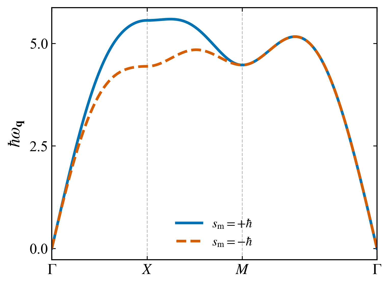
    01_spin_resolved_magnon_bands.png
        Spin/chirality-resolved magnon bands along Gamma-X-M-Gamma.

    02_chiral_splitting_path.png
        Splitting omega_+ - omega_- along Gamma-X-M-Gamma.

    03_chiral_splitting_map.png
        d-wave splitting map in the 2D Brillouin zone.

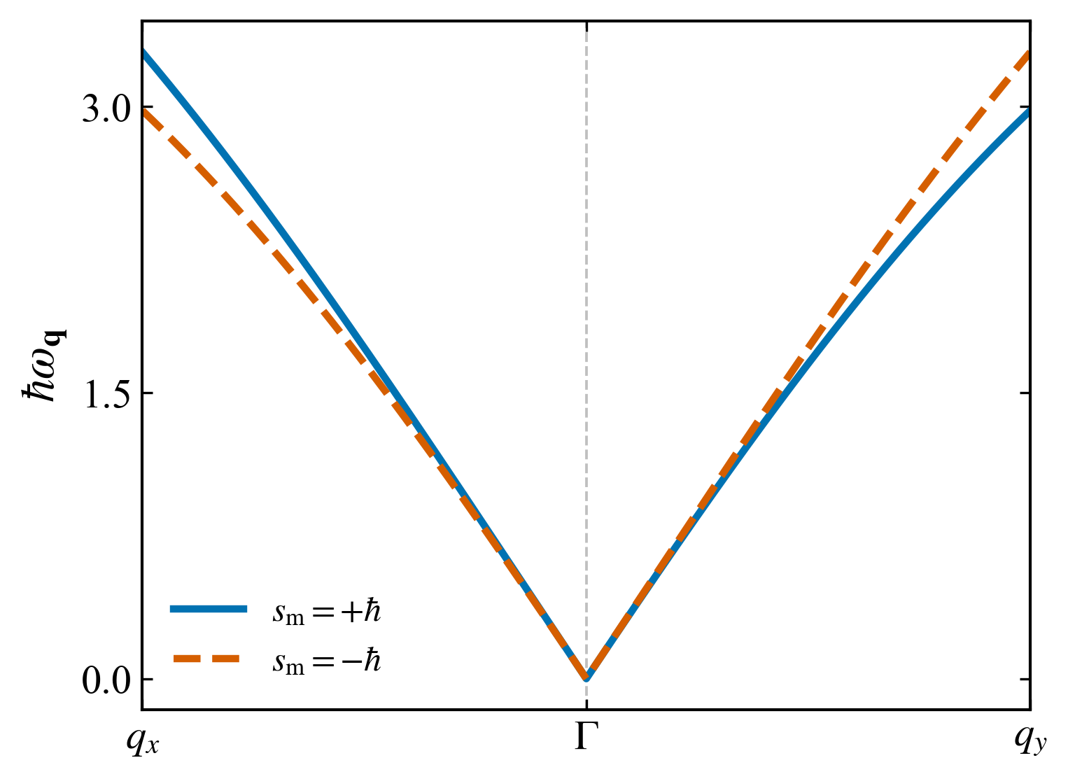
    04_near_gamma_spin_split_dispersion.png
        Near-Gamma split dispersion shown on a combined axis:
            left  side  -> Gamma to X  (q_y = 0, displayed as q_x side)
            right side  -> Gamma to Y  (q_x = 0, displayed as q_y side)
        Only the two split branches are plotted, so the sign reversal of the
        d-wave splitting becomes visually clear.

Model:
    A and B sublattices form a compensated collinear AFM.
    Nearest-neighbor A-B exchange is antiferromagnetic: J1 > 0.
    Same-sublattice exchange is treated as spin stiffness and is anisotropic.
    The anisotropy pattern on B is rotated by 90 degrees relative to A.

Linear spin-wave Hamiltonian:

    H_sw = E0 + sum_q [
        A_A(q) a_q^† a_q
      + A_B(q) b_q^† b_q
      + B(q) (a_q b_-q + a_q^† b_-q^†)
    ]

with

    A_A(q) = z J1 S
             + 2 S [K_Ax (1 - cos qx) + K_Ay (1 - cos qy)] + h_gap

    A_B(q) = z J1 S
             + 2 S [K_Bx (1 - cos qx) + K_By (1 - cos qy)] + h_gap

    B(q)   = z J1 S gamma_q

    gamma_q = (cos qx + cos qy) / 2

d-wave altermagnetic exchange pattern:

    K_Ax = K0 + dK,    K_Ay = K0 - dK
    K_Bx = K0 - dK,    K_By = K0 + dK

Then

    omega_+(q) - omega_-(q) is proportional to cos(qy) - cos(qx),

which is the d-wave chiral magnon splitting.
"""

from pathlib import Path
import numpy as np
import matplotlib.pyplot as plt
from matplotlib.ticker import MaxNLocator


# =========================================================
# Global plotting controls
# =========================================================
OUT_DIR = Path("magnon_altermagnet_results")
FIG_DIR = OUT_DIR / "figures"
FIG_DIR.mkdir(parents=True, exist_ok=True)

USE_TEX = False

FONT_SIZE = 16
LINE_WIDTH = 2.5
AXIS_WIDTH = 1.0
DPI = 300

plt.rcParams.update({
    "text.usetex": USE_TEX,
    "font.family": "serif",
    "font.serif": ["Times New Roman", "Times", "DejaVu Serif"],
    "mathtext.fontset": "stix",
    "font.size": FONT_SIZE,
    "axes.labelsize": FONT_SIZE,
    "axes.titlesize": FONT_SIZE,
    "xtick.labelsize": FONT_SIZE - 2,
    "ytick.labelsize": FONT_SIZE - 2,
    "legend.fontsize": FONT_SIZE - 4,
    "axes.linewidth": AXIS_WIDTH,
    "xtick.direction": "in",
    "ytick.direction": "in",
    "xtick.top": True,
    "ytick.right": True,
    "savefig.bbox": "tight",
    "savefig.dpi": DPI,
})


# =========================================================
# Model parameters
# =========================================================
S = 1.0
J1 = 1.0       # AFM A-B exchange
K0 = 0.25      # average same-sublattice stiffness
dK = 0.14      # d-wave altermagnetic anisotropy; dK=0 restores ordinary AFM degeneracy
h_gap = 0.00   # optional uniform magnon gap
a_lat = 1.0
z = 4

# Near-Gamma plot settings
QMAX_GAMMA = 1.10
N_GAMMA = 601

# Colors and line styles
COLOR_PLUS = "#0072B2"    # blue
COLOR_MINUS = "#D55E00"   # orange
COLOR_SPLIT = "#009E73"   # green
COLOR_ZERO = "0.35"

LS_PLUS = "-"
LS_MINUS = "--"


# =========================================================
# Utilities
# =========================================================
def set_max_three_ticks(ax, x=True, y=True):
    """
    Limit major ticks to at most three.
    Do not use this on the high-symmetry path x-axis.
    """
    if x:
        ax.xaxis.set_major_locator(MaxNLocator(nbins=3))
    if y:
        ax.yaxis.set_major_locator(MaxNLocator(nbins=3))


def savefig(fig, name):
    """
    Save PNG only.
    """
    png_path = FIG_DIR / f"{name}.png"
    fig.savefig(png_path, dpi=DPI)
    print(f"Saved: {png_path}")


def positive_eigenvalue(matrix):
    """
    Return the positive bosonic BdG eigenvalue from the dynamical matrix.
    """
    evals = np.linalg.eigvals(matrix)
    evals = np.real_if_close(evals, tol=1000).real

    positive = evals[evals >= -1e-10]
    if len(positive) == 0:
        return np.max(evals)

    return np.max(positive)


# =========================================================
# Linear spin-wave Hamiltonian
# =========================================================
def exchange_parameters(K0=K0, dK=dK):
    """
    d-wave altermagnetic exchange-stiffness pattern:
        A sublattice: stronger stiffness along x
        B sublattice: stronger stiffness along y
    """
    K_Ax = K0 + dK
    K_Ay = K0 - dK
    K_Bx = K0 - dK
    K_By = K0 + dK
    return K_Ax, K_Ay, K_Bx, K_By


def coefficients(qx, qy, S=S, J1=J1, K0=K0, dK=dK, h_gap=h_gap):
    """
    Return A_A(q), A_B(q), B(q), A0(q), deltaA(q), gamma(q).
    q values are dimensionless if a_lat = 1.
    """
    K_Ax, K_Ay, K_Bx, K_By = exchange_parameters(K0, dK)

    cx = np.cos(qx * a_lat)
    cy = np.cos(qy * a_lat)

    gamma = 0.5 * (cx + cy)

    AA = (
        z * J1 * S
        + h_gap
        + 2.0 * S * (K_Ax * (1.0 - cx) + K_Ay * (1.0 - cy))
    )

    AB = (
        z * J1 * S
        + h_gap
        + 2.0 * S * (K_Bx * (1.0 - cx) + K_By * (1.0 - cy))
    )

    B = z * J1 * S * gamma

    A0 = 0.5 * (AA + AB)
    deltaA = 0.5 * (AA - AB)

    return AA, AB, B, A0, deltaA, gamma


def dynamic_matrix_plus(qx, qy):
    """
    Bosonic dynamical matrix for the Nambu block:
        Psi_+ = (a_q, b_-q^†)^T
    """
    AA, AB, B, _, _, _ = coefficients(qx, qy)
    return np.array([[AA, B], [-B, -AB]], dtype=float)


def dynamic_matrix_minus(qx, qy):
    """
    Bosonic dynamical matrix for the Nambu block:
        Psi_- = (b_q, a_-q^†)^T
    """
    AA, AB, B, _, _, _ = coefficients(qx, qy)
    return np.array([[AB, B], [-B, -AA]], dtype=float)


def magnon_energies(qx, qy):
    """
    Diagonalize the two bosonic BdG dynamical matrices.

    Returns
        omega_plus, omega_minus, spin_plus, spin_minus
    """
    omega_plus = positive_eigenvalue(dynamic_matrix_plus(qx, qy))
    omega_minus = positive_eigenvalue(dynamic_matrix_minus(qx, qy))

    spin_plus = +1.0
    spin_minus = -1.0

    return omega_plus, omega_minus, spin_plus, spin_minus


# =========================================================
# High-symmetry path
# =========================================================
def interpolate_path(points, n_per_segment=240):
    """
    Return kpts, xcoord, xticks for a piecewise linear path.
    """
    kpts = []
    xcoord = []
    xticks = [0.0]
    total = 0.0

    for iseg in range(len(points) - 1):
        start = np.array(points[iseg], dtype=float)
        end = np.array(points[iseg + 1], dtype=float)

        for j in range(n_per_segment):
            t = j / n_per_segment
            q = (1.0 - t) * start + t * end

            if kpts:
                total += np.linalg.norm(q - kpts[-1])

            kpts.append(q)
            xcoord.append(total)

        xticks.append(total + np.linalg.norm(end - kpts[-1]))

    kpts.append(np.array(points[-1], dtype=float))
    total += np.linalg.norm(kpts[-1] - kpts[-2])
    xcoord.append(total)
    xticks[-1] = total

    return np.array(kpts), np.array(xcoord), xticks


def compute_high_symmetry_bands():
    Gamma = (0.0, 0.0)
    X = (np.pi, 0.0)
    M = (np.pi, np.pi)

    kpts, xcoord, xticks = interpolate_path([Gamma, X, M, Gamma], n_per_segment=240)

    omega_p = np.zeros(len(kpts))
    omega_m = np.zeros(len(kpts))

    for i, (qx, qy) in enumerate(kpts):
        omega_p[i], omega_m[i], _, _ = magnon_energies(qx, qy)

    return kpts, xcoord, xticks, omega_p, omega_m


# =========================================================
# Plot 1: spin/chirality-resolved bands
# =========================================================
def plot_spin_resolved_bands():
    _, xcoord, xticks, omega_p, omega_m = compute_high_symmetry_bands()

    fig, ax = plt.subplots(figsize=(5.4, 4.0))

    ax.plot(
        xcoord, omega_p,
        color=COLOR_PLUS, lw=LINE_WIDTH, ls=LS_PLUS,
        label=r"$s_{\mathrm{m}}=+\hbar$",
    )
    ax.plot(
        xcoord, omega_m,
        color=COLOR_MINUS, lw=LINE_WIDTH, ls=LS_MINUS,
        label=r"$s_{\mathrm{m}}=-\hbar$",
    )

    for x in xticks:
        ax.axvline(x, color="0.75", lw=0.8, ls="--", zorder=0)

    ax.set_xlim(xcoord[0], xcoord[-1])
    ax.set_xticks(xticks)
    ax.set_xticklabels([r"$\Gamma$", r"$X$", r"$M$", r"$\Gamma$"])
    ax.set_ylabel(r"$\hbar\omega_{\mathbf{q}}$")
    ax.legend(frameon=False, loc="best")

    set_max_three_ticks(ax, x=False, y=True)

    fig.tight_layout()
    savefig(fig, "01_spin_resolved_magnon_bands")
    plt.close(fig)


# =========================================================
# Plot 2: splitting along high-symmetry path
# =========================================================
def plot_splitting_along_path():
    _, xcoord, xticks, omega_p, omega_m = compute_high_symmetry_bands()
    split = omega_p - omega_m

    fig, ax = plt.subplots(figsize=(5.4, 3.6))

    ax.plot(xcoord, split, color=COLOR_SPLIT, lw=LINE_WIDTH, ls="-")
    ax.axhline(0.0, color=COLOR_ZERO, lw=0.9, ls="--", zorder=0)

    for x in xticks:
        ax.axvline(x, color="0.75", lw=0.8, ls="--", zorder=0)

    ax.set_xlim(xcoord[0], xcoord[-1])
    ax.set_xticks(xticks)
    ax.set_xticklabels([r"$\Gamma$", r"$X$", r"$M$", r"$\Gamma$"])
    ax.set_ylabel(r"$\omega_{+}-\omega_{-}$")

    set_max_three_ticks(ax, x=False, y=True)

    fig.tight_layout()
    savefig(fig, "02_chiral_splitting_path")
    plt.close(fig)


# =========================================================
# Plot 3: splitting map in BZ
# =========================================================
def plot_splitting_map(nk=301):
    q = np.linspace(-np.pi, np.pi, nk)
    qx_grid, qy_grid = np.meshgrid(q, q, indexing="xy")

    split = np.zeros_like(qx_grid)

    for ix in range(nk):
        for iy in range(nk):
            op, om, _, _ = magnon_energies(qx_grid[iy, ix], qy_grid[iy, ix])
            split[iy, ix] = op - om

    vmax = np.max(np.abs(split))
    if vmax < 1e-12:
        vmax = 1.0

    fig, ax = plt.subplots(figsize=(4.8, 4.0))

    im = ax.imshow(
        split,
        origin="lower",
        extent=(-np.pi, np.pi, -np.pi, np.pi),
        cmap="RdBu_r",
        vmin=-vmax,
        vmax=vmax,
        interpolation="bicubic",
        aspect="equal",
    )

    ax.set_xlabel(r"$q_x$")
    ax.set_ylabel(r"$q_y$")

    ax.set_xticks([-np.pi, 0.0, np.pi])
    ax.set_xticklabels([r"$-\pi$", r"$0$", r"$\pi$"])
    ax.set_yticks([-np.pi, 0.0, np.pi])
    ax.set_yticklabels([r"$-\pi$", r"$0$", r"$\pi$"])

    cbar = fig.colorbar(im, ax=ax, shrink=0.82, pad=0.03)
    cbar.set_label(r"$\omega_{+}-\omega_{-}$")
    cbar.locator = MaxNLocator(nbins=3)
    cbar.update_ticks()

    fig.tight_layout()
    savefig(fig, "03_chiral_splitting_map")
    plt.close(fig)


# =========================================================
# Plot 4: near-Gamma split dispersion with left qx and right qy
# =========================================================
def plot_near_gamma_split_dispersion(qmax=QMAX_GAMMA, nq=N_GAMMA):
    """
    Build a combined near-Gamma axis:
        x < 0 : Gamma -> X direction, with q = (|x|, 0)
        x > 0 : Gamma -> Y direction, with q = (0, x)

    Only the two split branches are plotted. This makes the sign reversal of
    the d-wave splitting between qx and qy directions clearly visible.
    """
    x = np.linspace(-qmax, qmax, nq)

    omega_p = np.zeros_like(x)
    omega_m = np.zeros_like(x)

    for i, xx in enumerate(x):
        if xx < 0:
            qx = -xx
            qy = 0.0
        else:
            qx = 0.0
            qy = xx

        omega_p[i], omega_m[i], _, _ = magnon_energies(qx, qy)

    fig, ax = plt.subplots(figsize=(5.4, 4.0))

    ax.plot(
        x, omega_p,
        color=COLOR_PLUS, lw=LINE_WIDTH, ls=LS_PLUS,
        label=r"$s_{\mathrm{m}}=+\hbar$",
    )
    ax.plot(
        x, omega_m,
        color=COLOR_MINUS, lw=LINE_WIDTH, ls=LS_MINUS,
        label=r"$s_{\mathrm{m}}=-\hbar$",
    )

    ax.axvline(0.0, color="0.75", lw=0.9, ls="--", zorder=0)

    ax.set_xlim(-qmax, qmax)
    ax.set_xticks([-qmax, 0.0, qmax])
    ax.set_xticklabels([r"$q_x$", r"$\Gamma$", r"$q_y$"])

    ax.set_ylabel(r"$\hbar\omega_{\mathbf{q}}$")
    ax.legend(frameon=False, loc="best")

    set_max_three_ticks(ax, x=False, y=True)

    fig.tight_layout()
    savefig(fig, "04_near_gamma_spin_split_dispersion")
    plt.close(fig)


# =========================================================
# Summary and main
# =========================================================
def print_model_summary():
    K_Ax, K_Ay, K_Bx, K_By = exchange_parameters(K0, dK)

    print("\nMinimal d-wave altermagnetic magnon model")
    print("==========================================")
    print(f"S      = {S}")
    print(f"J1     = {J1}")
    print(f"K0     = {K0}")
    print(f"dK     = {dK}")
    print(f"h_gap  = {h_gap}")
    print("")
    print("Same-sublattice exchange pattern:")
    print(f"K_Ax = {K_Ax:.6f}, K_Ay = {K_Ay:.6f}")
    print(f"K_Bx = {K_Bx:.6f}, K_By = {K_By:.6f}")
    print("")
    print("Expected d-wave splitting:")
    print("omega_+(q) - omega_-(q) ∝ cos(q_y) - cos(q_x)")
    print("")
    print("Near-Gamma plot:")
    print("left side  = q_x direction (q_y = 0)")
    print("right side = q_y direction (q_x = 0)")
    print("")
    print(f"Figures saved to: {FIG_DIR.resolve()}")


def main():
    print_model_summary()

    plot_spin_resolved_bands()
    plot_splitting_along_path()
    plot_splitting_map(nk=301)
    plot_near_gamma_split_dispersion(qmax=QMAX_GAMMA, nq=N_GAMMA)

    print("\nDone.")

if __name__ == "__main__":
    main()

鉴于该网站分享的大都是学习笔记，作者水平有限，若发现有问题可以发邮件给我

• yxliphy@gmail.com

也非常欢迎喜欢分享的小伙伴投稿